Routing Algorithms 1 Outline Routing Algorithm Shortest Path

Routing Algorithms 1

Outline • Routing Algorithm • Shortest Path Routing • Flow Based Routing • Distance Vector Routing • Link State Routing 2

Properties Of Routing Algorithm Routing is the process of forwarding of a packet in a network so that it reaches its intended destination. • Correctness: The routing should be done properly and correctly so that the packets may reach their proper destination. • Simplicity: The routing should be done in a simple manner so that the overhead is as low as possible. With increasing complexity of the routing algorithms the overhead also increases. • Robustness: Once a major network becomes operative, it may be expected to run continuously for years without any failures. The algorithms designed for routing should be robust enough to handle hardware and software failures and should be able to cope with changes in the topology and traffic without requiring all jobs in all 3 hosts to be aborted and the network rebooted every time some router goes down.

• Stability: The routing algorithms should be stable under all possible circumstances. • Fairness: Every node connected to the network should get a fair chance of transmitting their packets. this is generally done on a first come first serve basis. • Optimality: The routing algorithms should be optimal in terms of throughput and minimizing mean packet delays. here there is a trade-off and one has to choose depending on his suitability. 4

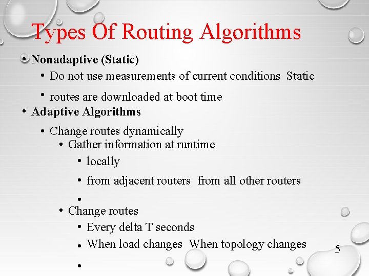
Types Of Routing Algorithms • Nonadaptive (Static) • Do not use measurements of current conditions Static • routes are downloaded at boot time • Adaptive Algorithms • Change routes dynamically • Gather information at runtime • locally • from adjacent routers from all other routers • • Change routes • Every delta T seconds • When load changes When topology changes • 5

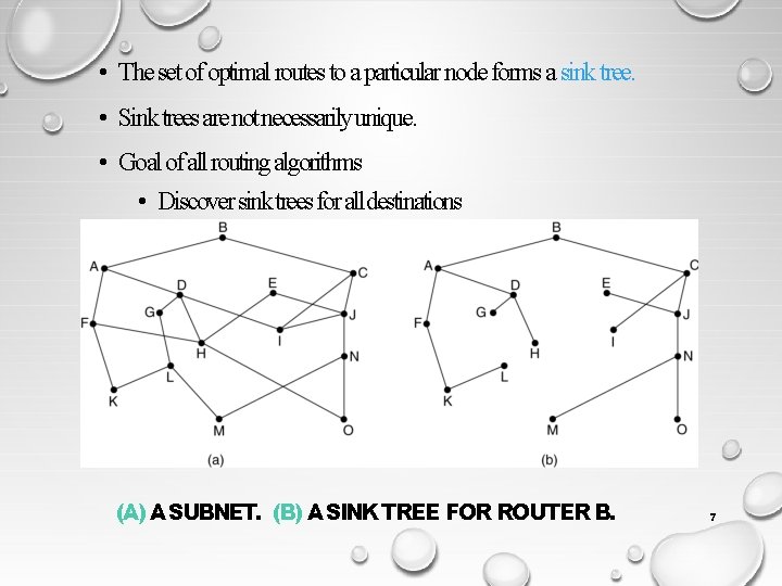
• The set of optimal routes to a particular node forms a sink tree. • Sink trees are not necessarilyunique. • Goal of all routing algorithms • Discover sink trees for alldestinations (A) A SUBNET. (B) A SINK TREE FOR ROUTER B. 7

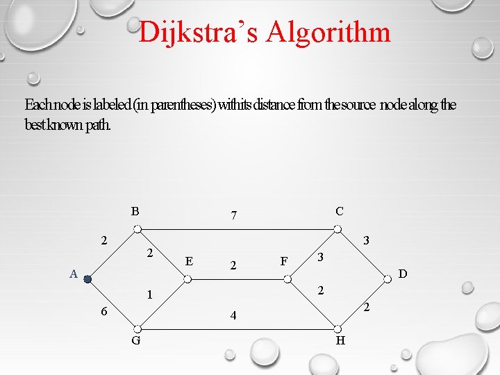
Dijkstra’s Algorithm Each node is labeled (in parentheses) withits distance from the source node along the best known path. B 2 2 A 3 E 2 F 3 D 2 1 6 C 7 2 4 G H

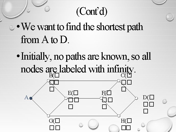
(Cont’d) • We want to find the shortest path from A to D. • Initially, no paths are known, so all nodes are labeled with infinity. B(� C(� �� � A G(� �� E(� �� � F(� �� � D(� �� � H(� ��

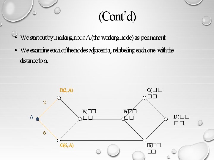
(Cont’d) • We startout by marking node A (the workingnode) as permanent. • We examine each of the nodes adjacent a, relabeling each one withthe distance to a. B(2, A) C(�� �� 2 E(�� �� A F(�� �� D(�� �� 6 G(6, A) H(�� ��

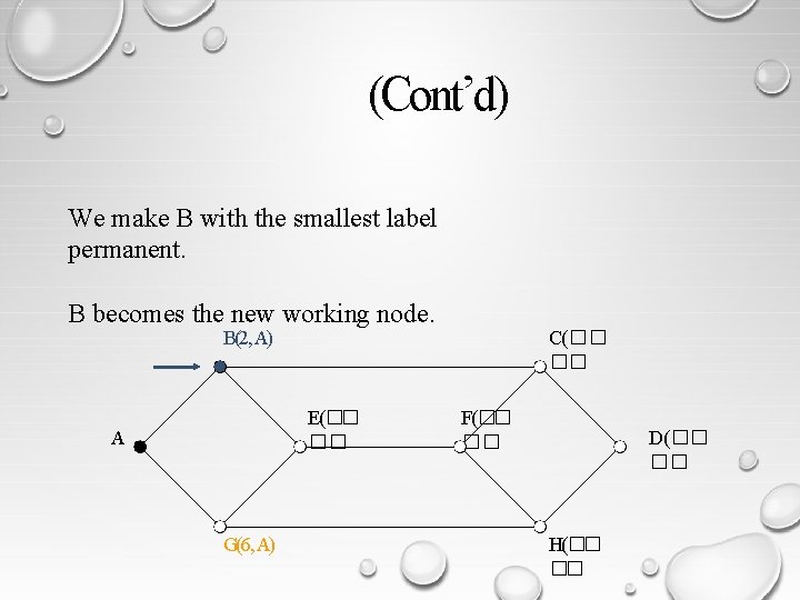
(Cont’d) We make B with the smallest label permanent. B becomes the new working node. B(2, A) E(�� �� A G(6, A) C(�� �� F(�� �� D(�� �� H(�� ��

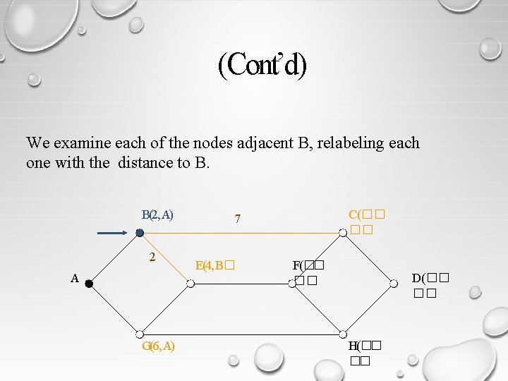
(Cont’d) We examine each of the nodes adjacent B, relabeling each one with the distance to B. B(2, A) 2 A G(6, A) C(�� �� 7 E(4, B� F(�� �� D(�� �� H(�� ��

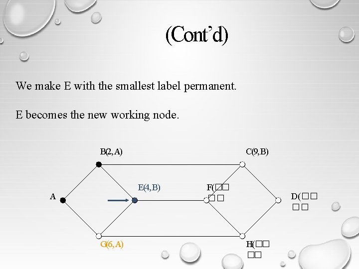
(Cont’d) We make E with the smallest label permanent. E becomes the new working node. B(2, A) C(9, B) E(4, B) A G(6, A) F(�� �� D(�� �� H(�� ��

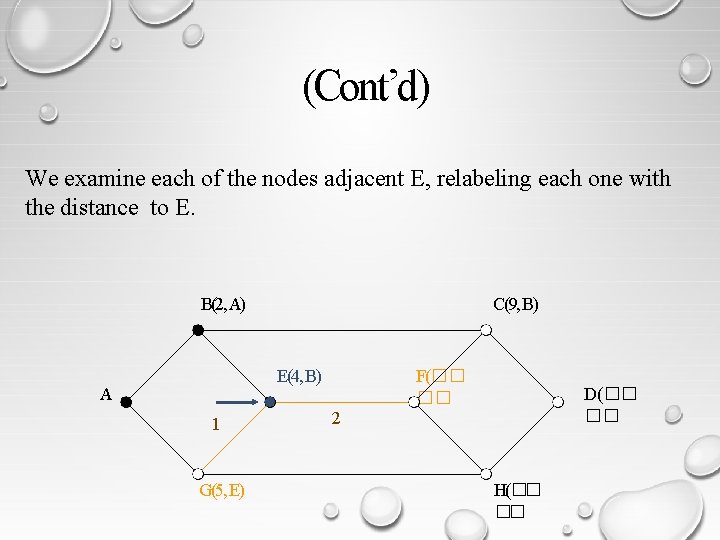
(Cont’d) We examine each of the nodes adjacent E, relabeling each one with the distance to E. B(2, A) C(9, B) E(4, B) A 1 G(5, E) F(�� �� D(�� �� 2 H(�� ��

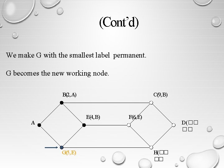
(Cont’d) We make G with the smallest label permanent. G becomes the new working node. B(2, A) C(9, B) E(4, B) A G(5, E) F(6, E) D(�� �� H(�� ��

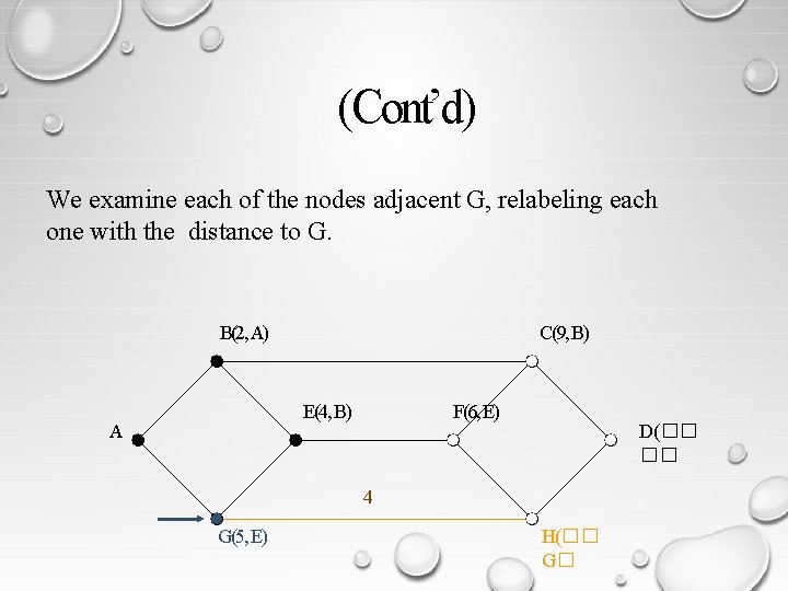
(Cont’d) We examine each of the nodes adjacent G, relabeling each one with the distance to G. B(2, A) C(9, B) E(4, B) A F(6, E) D(�� �� 4 G(5, E) H(�� G�

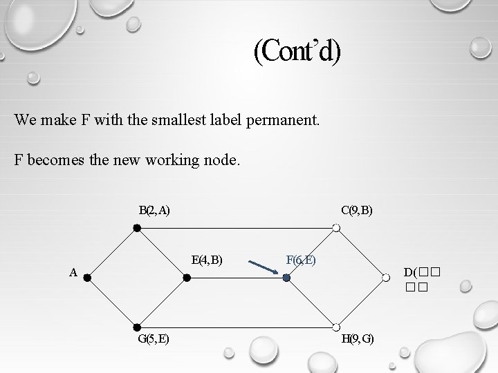
(Cont’d) We make F with the smallest label permanent. F becomes the new working node. B(2, A) C(9, B) E(4, B) A G(5, E) F(6, E) D(�� �� H(9, G)

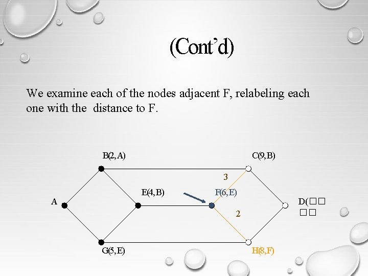
(Cont’d) We examine each of the nodes adjacent F, relabeling each one with the distance to F. B(2, A) C(9, B) 3 E(4, B) A F(6, E) D(�� �� 2 G(5, E) H(8, F)

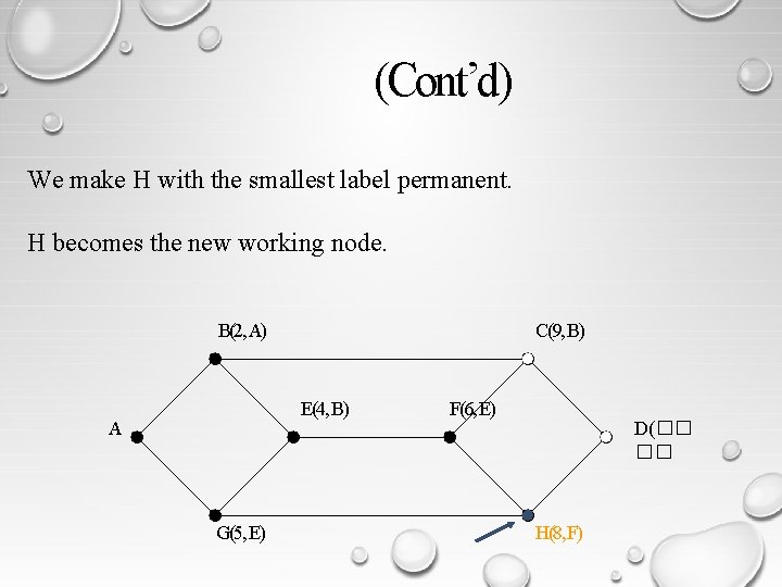
(Cont’d) We make H with the smallest label permanent. H becomes the new working node. B(2, A) C(9, B) E(4, B) A G(5, E) F(6, E) D(�� �� H(8, F)

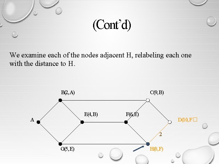
(Cont’d) We examine each of the nodes adjacent H, relabeling each one with the distance to H. B(2, A) C(9, B) E(4, B) A F(6, E) D(10, F� 2 G(5, E) H(8, F)

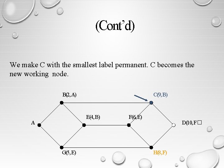
(Cont’d) We make C with the smallest label permanent. C becomes the new working node. B(2, A) C(9, B) E(4, B) A G(5, E) F(6, E) D(10, F� H(8, F)

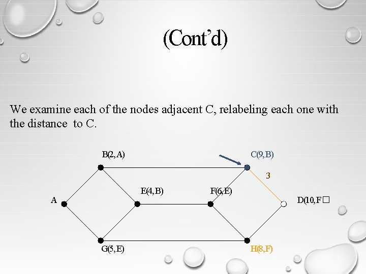
(Cont’d) We examine each of the nodes adjacent C, relabeling each one with the distance to C. B(2, A) C(9, B) 3 E(4, B) A G(5, E) F(6, E) D(10, F� H(8, F)

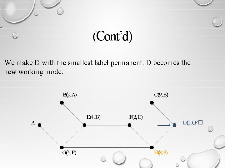
(Cont’d) We make D with the smallest label permanent. D becomes the new working node. B(2, A) C(9, B) E(4, B) A G(5, E) F(6, E) D(10, F� H(8, F)

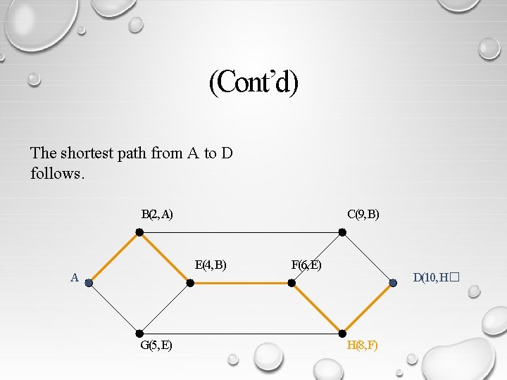
(Cont’d) The shortest path from A to D follows. B(2, A) C(9, B) E(4, B) A G(5, E) F(6, E) D(10, H� H(8, F)

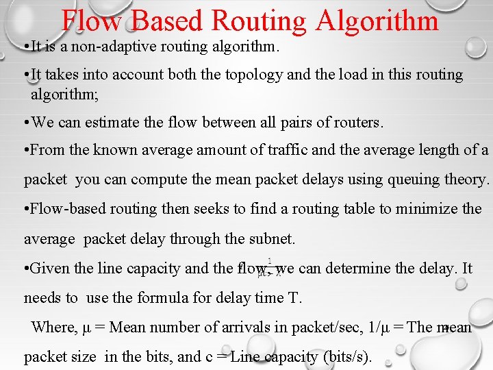
Flow Based Routing Algorithm • It is a non-adaptive routing algorithm. • It takes into account both the topology and the load in this routing algorithm; • We can estimate the flow between all pairs of routers. • From the known average amount of traffic and the average length of a packet you can compute the mean packet delays using queuing theory. • Flow-based routing then seeks to find a routing table to minimize the average packet delay through the subnet. • Given the line capacity and the flow, we can determine the delay. It needs to use the formula for delay time T. 24 Where, μ = Mean number of arrivals in packet/sec, 1/μ = The mean packet size in the bits, and c = Line capacity (bits/s).

Routing: Distance Vector • Adaptive algorithm • Exchange of info only with neighbours • Data to be available in each router • Routing table: per destination • Distance • Outgoing line • Distance to all neighbours 25

• Algorithm • At each step within a router: • Get routing tables from neighbours • Compute distance to neighbours • Compute new routing table 26

Routing: Link State • Each router must • Discover its neighbours and learn their network addresses • Measure the delay or cost to each of its neighbours • Construct a packet with these distances • Send this packet to all other routers • Compute the shortest path to every other router 27

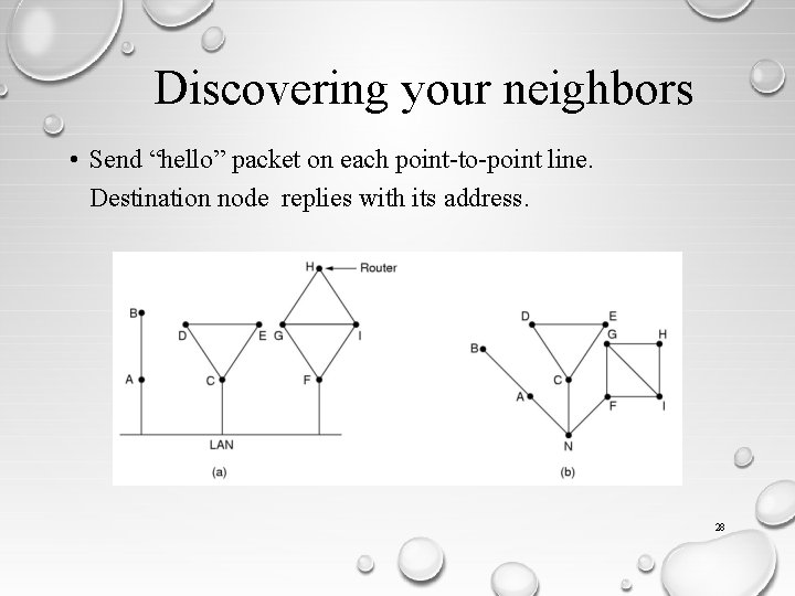
Discovering your neighbors • Send “hello” packet on each point-to-point line. Destination node replies with its address. 28

Measuring line cost • Send an “ECHO” packet over the line. • Destination is required to respond to “echo” packet immediately. • Measure the time required for this operation. 29

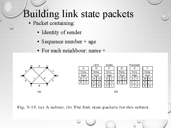
Building link state packets • Packet containing: • Identity of sender • Sequence number + age • For each neighbour: name + distance 43

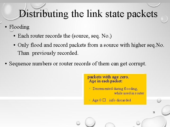
Distributing the link state packets • Flooding • Each router records the (source, seq. No. ) • Only flood and record packets from a source with higher seq. No. Than previously recorded. • Sequence numbers or router records of them can get corrupt. packets with age zero. Age in each packet: • Decremented during flooding, while used in router • Age 0 � info discarded 31

Computing new routes • With a full set of link state packets, a router can: • Construct the entire subnet graph • Run Dijkstra's algorithm to compute the shortest path to each destination • Problems for large subnets • Memory to store data • Compute time 32

Thank you 33