Risk Analysis Modelling Lecture 3 Constrained Efficient Frontiers

Risk Analysis & Modelling Lecture 3: Constrained Efficient Frontiers

http: //www. angelfire. com/linux/lecturenotes

What We Will Look At In This Lecture • • • The importance of the concept of return Another look at investment ‘weights’ The concept of the efficient frontier The calculation of the unconstrained frontier The calculation of the constrained frontier The use of Excel Solver to perform constrained optimisation

Important Concepts From Last Week • Some variables are ‘random’ and have uncertainty or ‘risk’ • We decided that the mean and the variance might be good measures for risk and return • The mean and variance of a portfolio of assets can be ‘implied’ from the mean, variance and covariance of the assets it contains

The Return Of An Asset • Last week we talked about the return of a portfolio in terms of the return of its assets • When we talk about returns we are talking about proportional changes in the value of an asset or portfolio • Using returns allow us to simplify the problem because it allows us to think of all assets in a similar way regardless of their physical size • This size independence simplifies the problem we face in quantifying risk since we can ‘compare’ assets of different sizes

2 Equally Likable Investments • Investment 1 consists of buying stocks at £ 10 each of which will be worth £ 11 in one year • Investment 2 consists of buying houses for £ 100, 000 each of which will be worth £ 110, 000 in one year • If we have £ 1, 000 to invest should we buy 10 houses or 100, 000 stocks? • What we care about is the proportional return or growth in our investments not the absolute size of their gains • The same is also true of our liabilities (like the rate of interest your bank charges you)

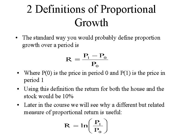
2 Definitions of Proportional Growth • The standard way you would probably define proportion growth over a period is • Where P(0) is the price in period 0 and P(1) is the price in period 1 • Using this definition the return for both the house and the stock would be 10% • Later in the course we will see why a different but related measure of proportional return is useful:

An Interesting Question • If we accept the basic assumptions that we can parameterise investments (and liabilities) in terms of the mean (good) and standard deviation (bad) of their returns. Then an interesting question arises: What is the portfolio with the highest expected return for a given deviation? • As we saw in last weeks exercise the behaviour of risk is complicated by the quadratic nature of the variance of a portfolio in terms of the assets it contains. (The quadratic relationship means that more than one portfolio can have the same risk, so we have a choice)

Std. Dev[RP] E[RP] The Efficient Frontier For The 2 Asset Case Max Return Portfolio y 1. 0 x y Minimum Variance E[RP] x WA Max Return Portfolio Efficient portfolio (WA = y) Inefficient portfolio (WA = x) Std. Dev[RP] WA

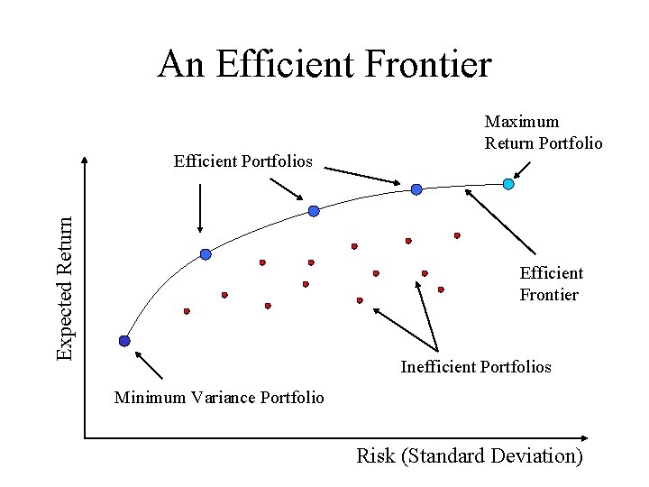
Observations From The 2 Asset Case • There can be 2 possible portfolios for a given level of risk due to the quadratic nature of variance • Although these portfolios have the same variance one can have a higher return than the other, and is thus more efficient • The highest return portfolio will contain 100% in the asset with the highest return • The minimum return portfolio can be determined from just looking at the variance chart • The ‘efficient’ part of the curve (the efficient frontier) is bounded between the minimum variance portfolio and the max return portfolio

Optimising Portfolios With More Than 2 Assets • For portfolios containing 3 assets or more there are no simple graphical representations • The two asset case is simple because we only have one choice variable (ie investment in asset A, the investment in the second asset is then implied) • We must rely entirely on mathematics to solve problems of 3 assets or more • Many of the insights we observed for the 2 assets are true for all fontiers • We will used Excel’s solver to calculate the optimal portfolios and the efficient frontier

An Efficient Frontier Expected Return Efficient Portfolios Maximum Return Portfolio Efficient Frontier Inefficient Portfolios Minimum Variance Portfolio Risk (Standard Deviation)

General Description Of The Problem • • Minimise the Var[Rp] Where E[RP] = WT. R Var[RP] = WT. C. W Subject to We. F F is the set (or group) of feasible weight vectors, e comes from set notation and means belongs to. So W e F means the weight vector must belong to the set of feasible vectors (or feasible regions)

The 2 Asset Case In This Notation • Minimise the Var[Rp] Where E[RP] = WT. R Var[RP] = WT. C. W Subject to We. F where F is the set of all vectors for which WA+WB=1, 0<=WA<=1, 0<=WB<=1 and E[Rp] = T • Where T is our target return.

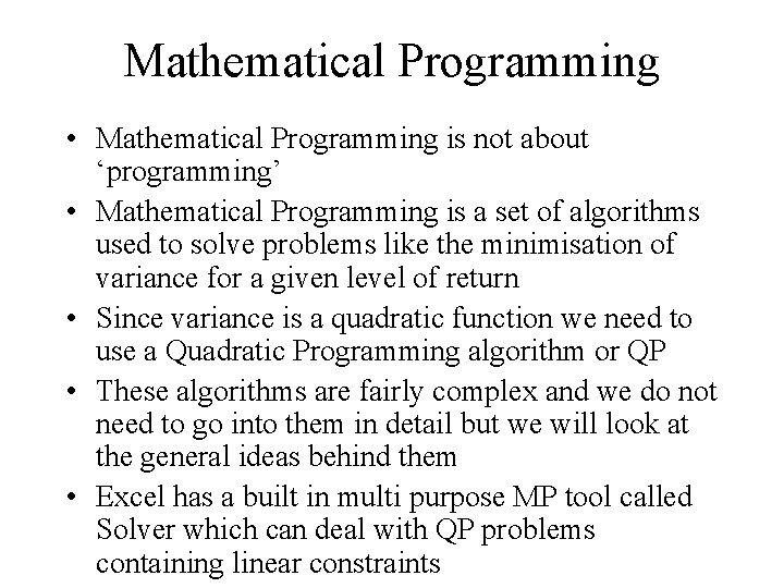
Mathematical Programming • Mathematical Programming is not about ‘programming’ • Mathematical Programming is a set of algorithms used to solve problems like the minimisation of variance for a given level of return • Since variance is a quadratic function we need to use a Quadratic Programming algorithm or QP • These algorithms are fairly complex and we do not need to go into them in detail but we will look at the general ideas behind them • Excel has a built in multi purpose MP tool called Solver which can deal with QP problems containing linear constraints

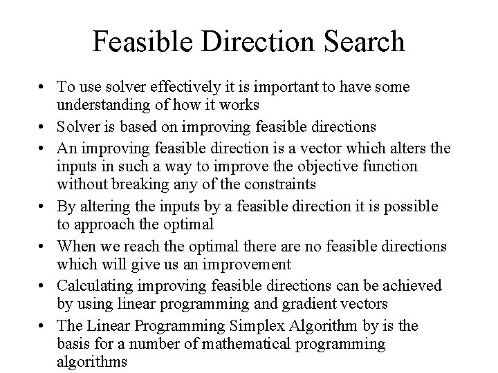
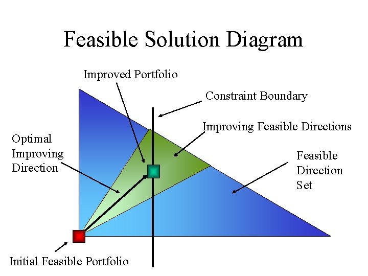
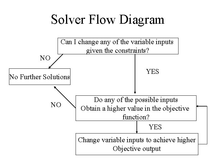
Feasible Direction Search • To use solver effectively it is important to have some understanding of how it works • Solver is based on improving feasible directions • An improving feasible direction is a vector which alters the inputs in such a way to improve the objective function without breaking any of the constraints • By altering the inputs by a feasible direction it is possible to approach the optimal • When we reach the optimal there are no feasible directions which will give us an improvement • Calculating improving feasible directions can be achieved by using linear programming and gradient vectors • The Linear Programming Simplex Algorithm by is the basis for a number of mathematical programming algorithms

Feasible Solution Diagram Improved Portfolio Constraint Boundary Optimal Improving Direction Initial Feasible Portfolio Improving Feasible Directions Feasible Direction Set

Solver Flow Diagram NO Can I change any of the variable inputs given the constraints? No Further Solutions NO YES Do any of the possible inputs Obtain a higher value in the objective function? YES Change variable inputs to achieve higher Objective output

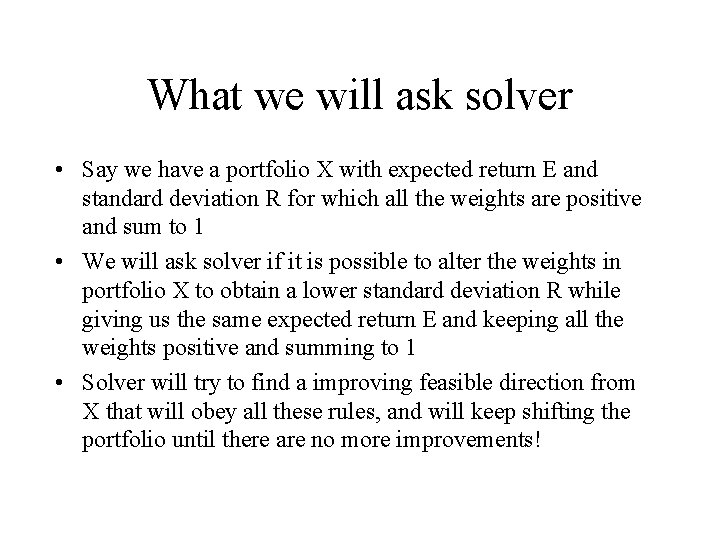
What we will ask solver • Say we have a portfolio X with expected return E and standard deviation R for which all the weights are positive and sum to 1 • We will ask solver if it is possible to alter the weights in portfolio X to obtain a lower standard deviation R while giving us the same expected return E and keeping all the weights positive and summing to 1 • Solver will try to find a improving feasible direction from X that will obey all these rules, and will keep shifting the portfolio until there are no more improvements!

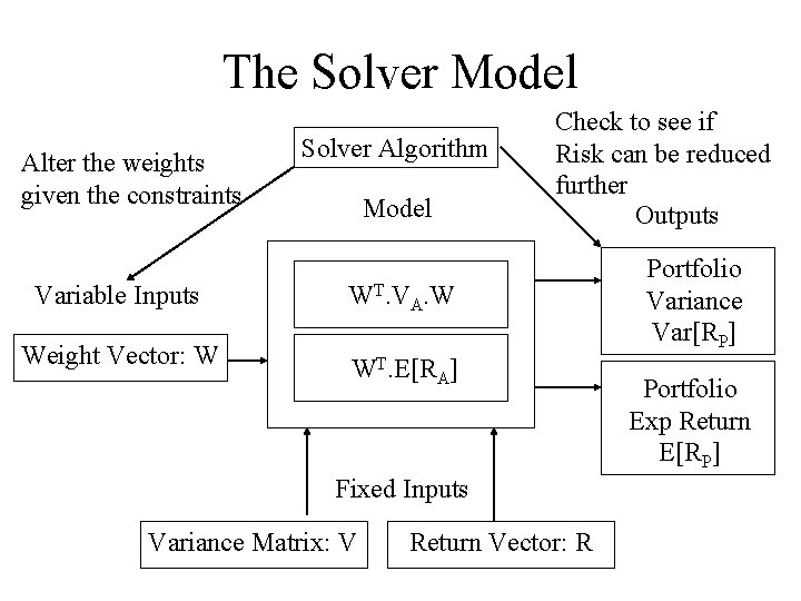
The Solver Model Alter the weights given the constraints Solver Algorithm Model Variable Inputs WT. VA. W Weight Vector: W WT. E[RA] Check to see if Risk can be reduced further Outputs Fixed Inputs Variance Matrix: V Return Vector: R Portfolio Variance Var[RP] Portfolio Exp Return E[RP]

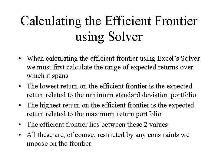
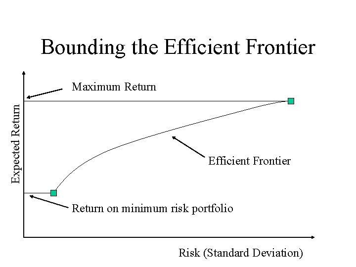
Calculating the Efficient Frontier using Solver • When calculating the efficient frontier using Excel’s Solver we must first calculate the range of expected returns over which it spans • The lowest return on the efficient frontier is the expected return related to the minimum standard deviation portfolio • The highest return on the efficient frontier is the expected return related to the maximum return portfolio • The efficient frontier lies between these 2 values • All these are, of course, restricted by any constraints we impose on the frontier

Bounding the Efficient Frontier Expected Return Maximum Return Efficient Frontier Return on minimum risk portfolio Risk (Standard Deviation)

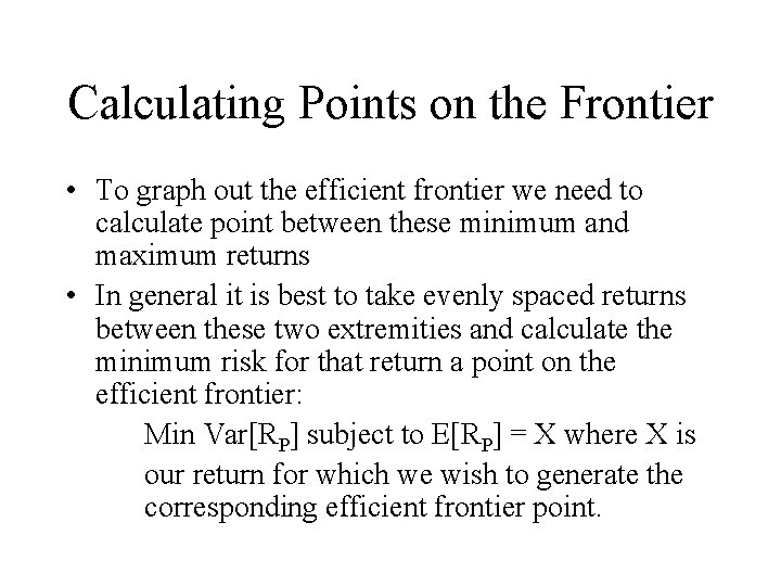
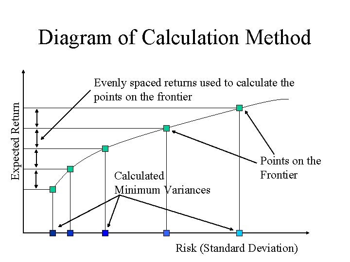
Calculating Points on the Frontier • To graph out the efficient frontier we need to calculate point between these minimum and maximum returns • In general it is best to take evenly spaced returns between these two extremities and calculate the minimum risk for that return a point on the efficient frontier: Min Var[RP] subject to E[RP] = X where X is our return for which we wish to generate the corresponding efficient frontier point.

Expected Return Diagram of Calculation Method Evenly spaced returns used to calculate the points on the frontier Calculated Minimum Variances Points on the Frontier Risk (Standard Deviation)

Where do I Find Solver • Solver comes as standard with Excel and is an Excel Add-in • It is found under Tools->Solver • If it is not available then you might need to tell Excel to load it by going to Tools->Addins and making sure the “Solver Add-in” is checked • Solver is programmed in VBA!

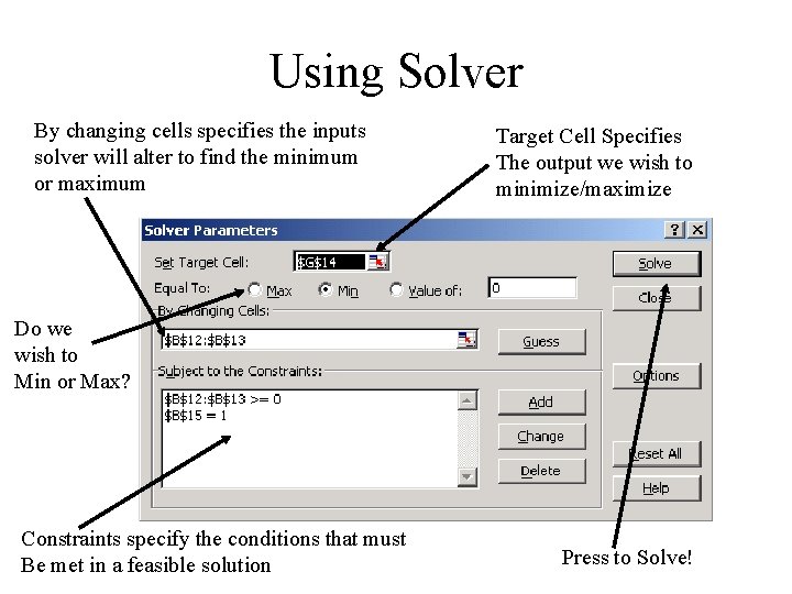
Using Solver By changing cells specifies the inputs solver will alter to find the minimum or maximum Target Cell Specifies The output we wish to minimize/maximize Do we wish to Min or Max? Constraints specify the conditions that must Be met in a feasible solution Press to Solve!

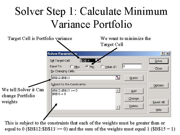
Solver Step 1: Calculate Minimum Variance Portfolio Target Cell is Portfolio variance We want to minimize the Target Cell We tell Solver it Can change Portfolio weights This is subject to the constraints that each of the weights must be greater than or equal to 0 ($B$12: $B$13 >= 0) and the sum of the weights must equal 1 ($B$15 = 1)

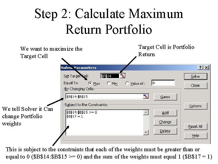
Step 2: Calculate Maximum Return Portfolio We want to maximize the Target Cell is Portfolio Return We tell Solver it Can change Portfolio weights This is subject to the constraints that each of the weights must be greater than or equal to 0 ($B$14: $B$15 >= 0) and the sum of the weights must equal 1 ($B$17 = 1)

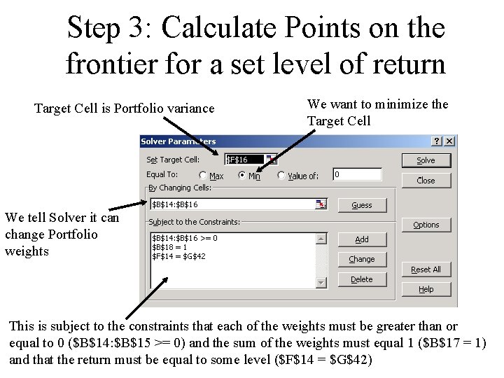
Step 3: Calculate Points on the frontier for a set level of return Target Cell is Portfolio variance We want to minimize the Target Cell We tell Solver it can change Portfolio weights This is subject to the constraints that each of the weights must be greater than or equal to 0 ($B$14: $B$15 >= 0) and the sum of the weights must equal 1 ($B$17 = 1) and that the return must be equal to some level ($F$14 = $G$42)

Our Efficient Frontier Algorithm 1) 2) 3) 4) 5) Use solver step 1 to calculate the minimum variance portfolio and save its risk and return values (by copy and paste) Use solver step 2 to calculate the maximum return portfolio and save its risk and return values Take evenly spaced returns between the values calculated in 1) and 2) and use solver step 3 to calculate their associated efficient frontier values saving each risk and return pair Copy and Paste the mean and variance of portfolio return into a table (using Paste Special, Values) Graph out all risk return pairs to view the efficient frontier

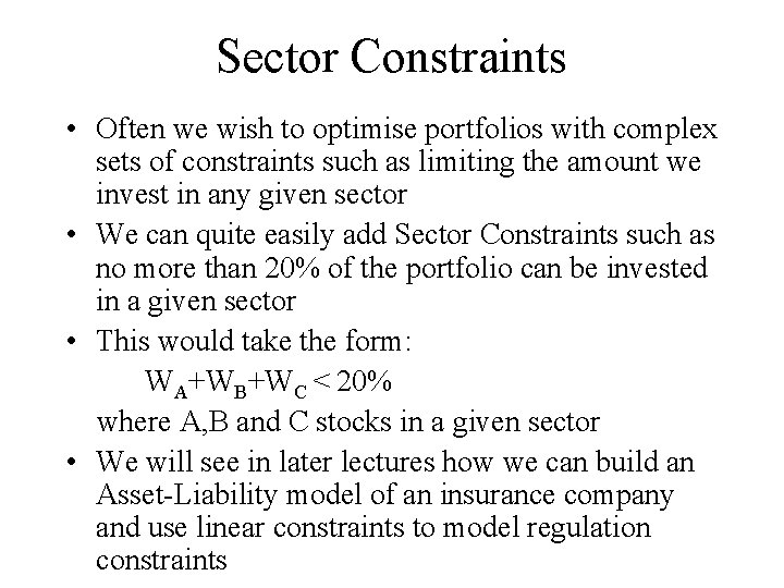
Sector Constraints • Often we wish to optimise portfolios with complex sets of constraints such as limiting the amount we invest in any given sector • We can quite easily add Sector Constraints such as no more than 20% of the portfolio can be invested in a given sector • This would take the form: WA+WB+WC < 20% where A, B and C stocks in a given sector • We will see in later lectures how we can build an Asset-Liability model of an insurance company and use linear constraints to model regulation constraints

What if you like risk? • An interesting question is does the efficient frontier analysis apply if you like risk? • Would you still want to minimize risk for a given level of return? • The answer is yes: “Minimise Risk for a given level of return” has an equivalent “Optimise return for a given level of risk” • This is called the ‘Dual’ • So for a given level of risk the efficient frontier also gives us the best return • Efficient portfolios are said to be stochastically dominant to inefficient portfolios

The Dual • For every constrained maximisation problem there is an equivalent constrained minimisation problem called the Dual • So far we have been saying maximise the risk for a given level of return • The dual of this is to maximise return for a given level of risk • Investors often have target returns and want to know how much risk they must incur • But they could equally well have a risk threshold and want to know what the maximum return they could obtain