Decision and Risk Analysis Financial Modelling Risk Analysis

Decision and Risk Analysis Financial Modelling & Risk Analysis II Kiriakos Vlahos Spring 2000

Session overview • Probability distributions for Risk Analysis – Subjective – Regression and Forecasting models – Historic data • Resampling • Distribution fitting • Sampling distributions – Using histograms – The inversion method • Correlated random variables • Comparing uncertain outcomes – Dynatron case

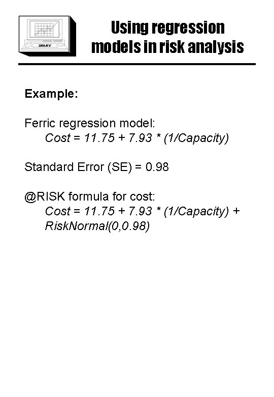
Using regression models in risk analysis Example: Ferric regression model: Cost = 11. 75 + 7. 93 * (1/Capacity) Standard Error (SE) = 0. 98 @RISK formula for cost: Cost = 11. 75 + 7. 93 * (1/Capacity) + Risk. Normal(0, 0. 98)

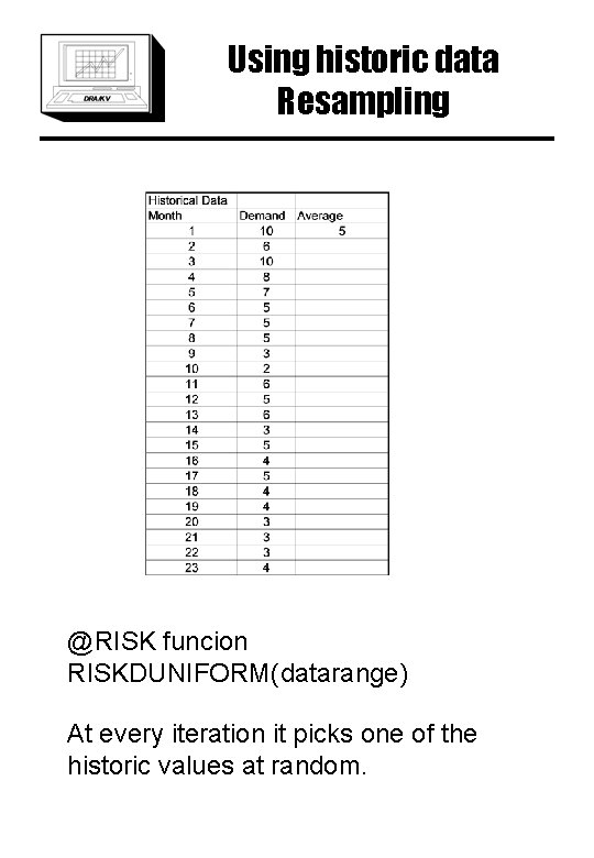
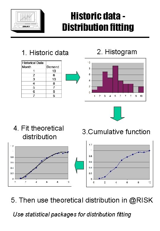
Using historic data Resampling @RISK funcion RISKDUNIFORM(datarange) At every iteration it picks one of the historic values at random.

Historic data Distribution fitting 1. Historic data 4. Fit theoretical distribution 2. Histogram 3. Cumulative function 5. Then use theoretical distribution in @RISK Use statistical packages for distribution fitting

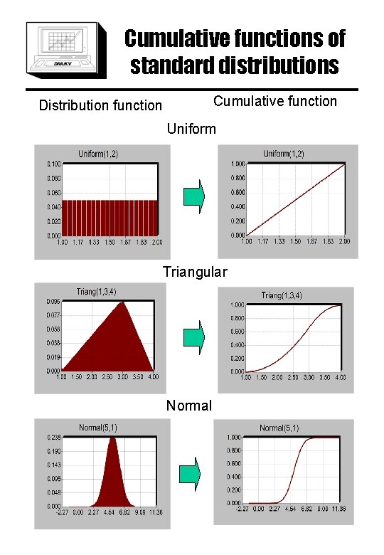
Cumulative functions of standard distributions Cumulative function Distribution function Uniform Triangular Normal

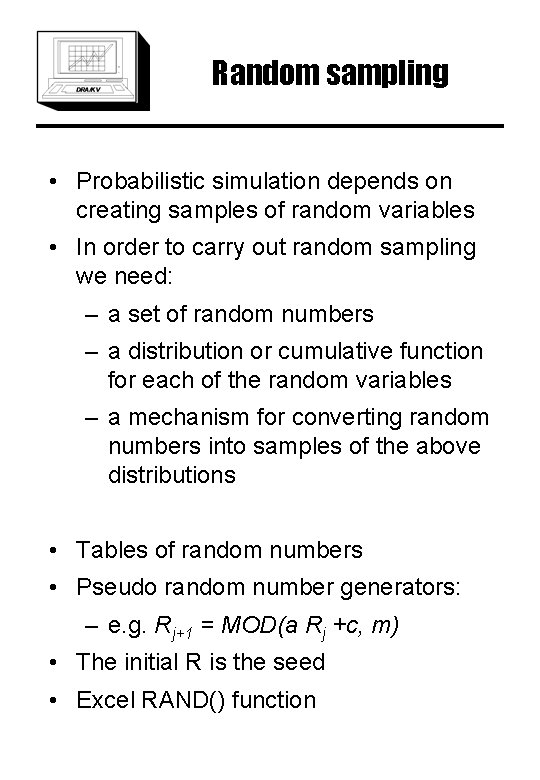
Random sampling • Probabilistic simulation depends on creating samples of random variables • In order to carry out random sampling we need: – a set of random numbers – a distribution or cumulative function for each of the random variables – a mechanism for converting random numbers into samples of the above distributions • Tables of random numbers • Pseudo random number generators: – e. g. Rj+1 = MOD(a Rj +c, m) • The initial R is the seed • Excel RAND() function

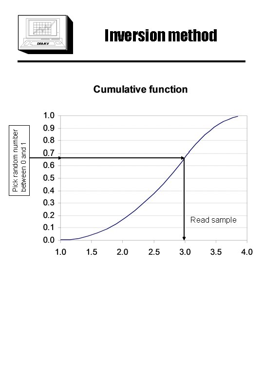
Pick random number between 0 and 1 Inversion method Read sample

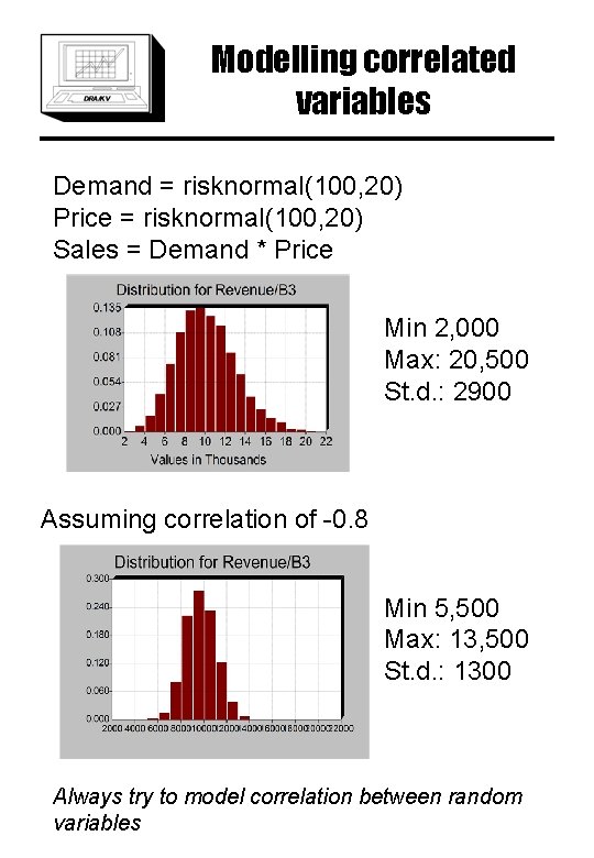
Modelling correlated variables Demand = risknormal(100, 20) Price = risknormal(100, 20) Sales = Demand * Price Min 2, 000 Max: 20, 500 St. d. : 2900 Assuming correlation of -0. 8 Min 5, 500 Max: 13, 500 St. d. : 1300 Always try to model correlation between random variables

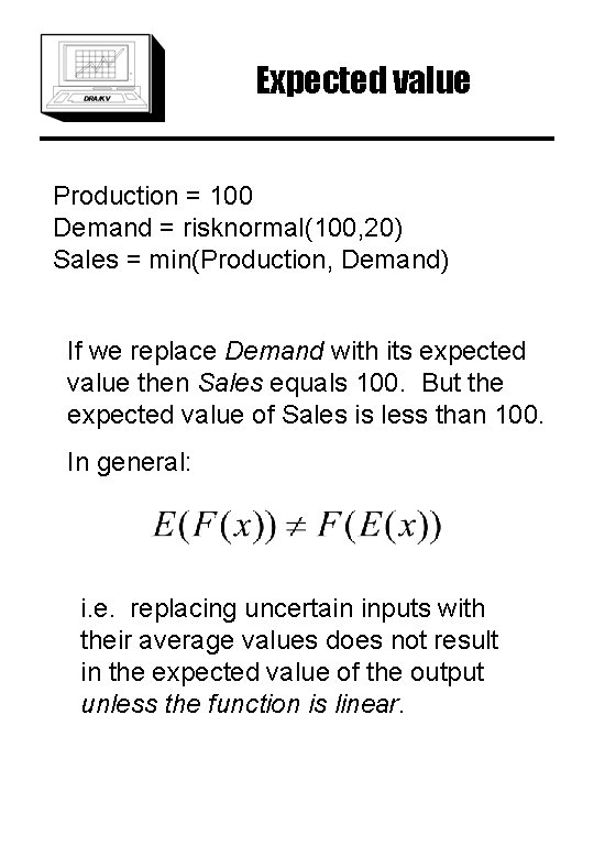
Expected value Production = 100 Demand = risknormal(100, 20) Sales = min(Production, Demand) If we replace Demand with its expected value then Sales equals 100. But the expected value of Sales is less than 100. In general: i. e. replacing uncertain inputs with their average values does not result in the expected value of the output unless the function is linear.

Dynatron • Decide about: – The production level of Dynatron toys – the split into super and standard

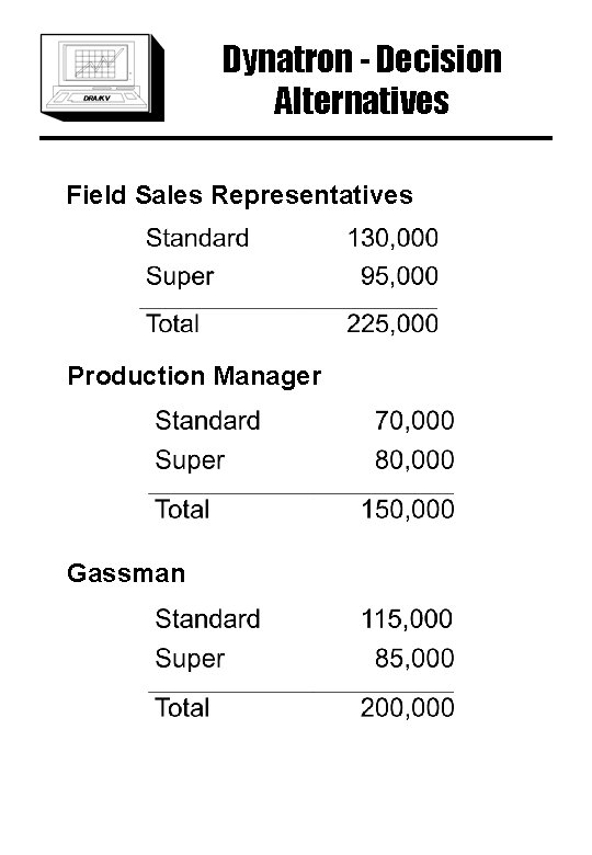
Dynatron - Decision Alternatives Field Sales Representatives Production Manager Gassman

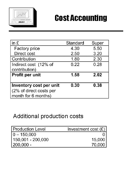
Cost Accounting Additional production costs

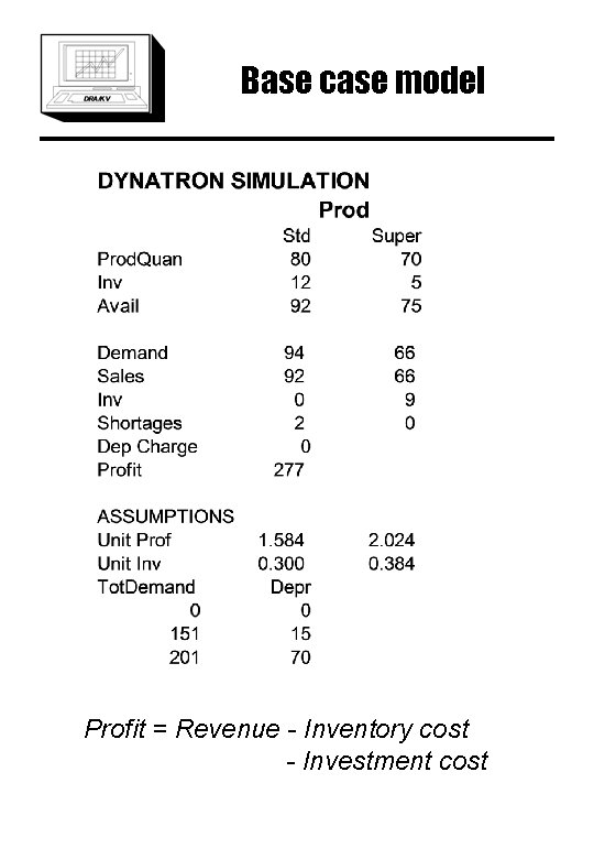
Base case model Profit = Revenue - Inventory cost - Investment cost

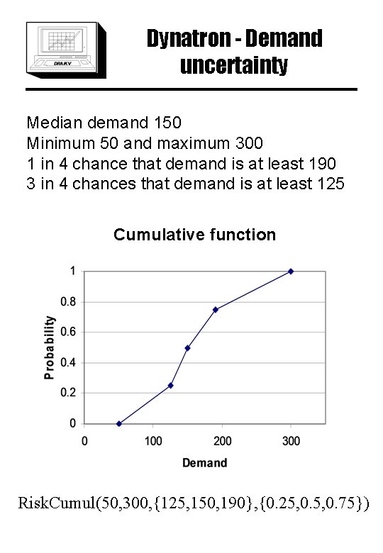
Dynatron - Demand uncertainty Median demand 150 Minimum 50 and maximum 300 1 in 4 chance that demand is at least 190 3 in 4 chances that demand is at least 125 Cumulative function Risk. Cumul(50, 300, {125, 150, 190}, {0. 25, 0. 75})

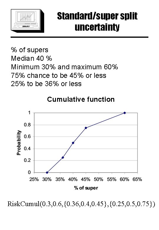
Standard/super split uncertainty % of supers Median 40 % Minimum 30% and maximum 60% 75% chance to be 45% or less 25% to be 36% or less Cumulative function Risk. Cumul(0. 3, 0. 6, {0. 36, 0. 45}, {0. 25, 0. 75})

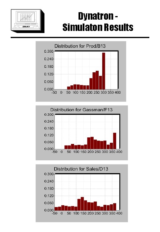
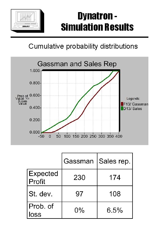
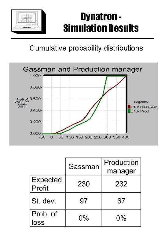
Dynatron Simulaton Results

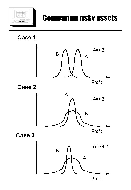
Comparing risky assets Case 1 A>>B B A Profit Case 2 A A>>B B Profit Case 3 A>>B ? B A Profit

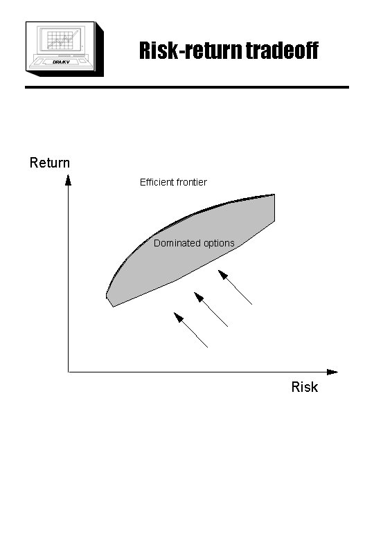
Risk-return tradeoff Return Efficient frontier Dominated options Risk

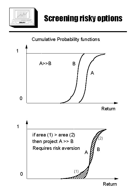
Screening risky options Cumulative Probability functions 1 A>>B B A 0 Return 1 if area (1) > area (2) then project A >> B Requires risk aversion 0 (2) A B (1) Return

Dynatron Simulation Results Cumulative probability distributions

Dynatron Simulation Results Cumulative probability distributions

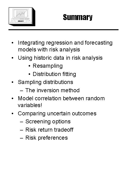
Summary • Integrating regression and forecasting models with risk analysis • Using historic data in risk analysis • Resampling • Distribution fitting • Sampling distributions – The inversion method • Model correlation between random variables! • Comparing uncertain outcomes – Screening options – Risk return tradeoff – Risk preferences