FINANCIAL ENGINEERING DERIVATIVES AND RISK MANAGEMENT J Wiley

FINANCIAL ENGINEERING: DERIVATIVES AND RISK MANAGEMENT (J. Wiley, 2001) K. Cuthbertson and D. Nitzsche Lecture Pricing Interest Rate Derivatives © K. Cuthbertson, D. Nitzsche

TOPICS Equilibrium Models pricing a zero, under stochastic interest rates No-Arbitrage Approach and the BOPM pricing coupon bonds, bond options, callable bonds, FRN’s, caps and FRA’s Pricing using Monte Carlo Simulation

EQUILIBRIUM MODELS Choose a continuous time formulation for the short rate process and estimate the unknown parameters of this process, from historic data on spot rates. Mathematically derive the whole term structure from the chosen short rate model. Use continuous time mathematics to establish the PDE for the interest rate derivative under consideration Solve this PDE to give a closed form solution for the price of the derivative in terms of the estimated parameters of the short rate model.

EQUILIBRIUM MODELS RNV Model for short rate [18. 31] dr = (r, t) dt + (r, t) Ho-Lee model [18. 44] B-S, PDE dr = a dt +

Price a Zero, under stochastic interest rates Trial soln to BS, PDE [18. 45] f(t, T) = k(t, T) exp{-r(T-t)} Substituting the derivatives of [18. 45] into B-S, PDE and integrating, we obtain closed form solution [18. 47] ln(k(t, T)) = -(1/2) (T-t)2 a + (1/6) (T-t)3 2 Sub soln for P(t, T) in long-rate equation: [18. 48] Ho-Lee model only allows a parallel shift in the yield curve. Rather restrictive term structure: ameliorated by using alternative stochastic process for the short rate

No-Arbitrage Approach and the BOPM

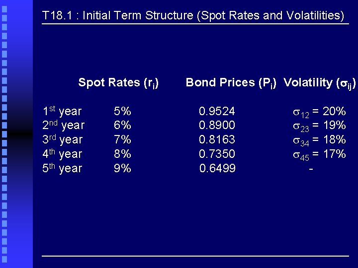
T 18. 1 : Initial Term Structure (Spot Rates and Volatilities) Spot Rates (ri) 1 st year 2 nd year 3 rd year 4 th year 5% 6% 7% 8% 9% Bond Prices (Pi) Volatility (sij) 0. 9524 0. 8900 0. 8163 0. 7350 0. 6499 12 = 20% 23 = 19% 34 = 18% 45 = 17% -

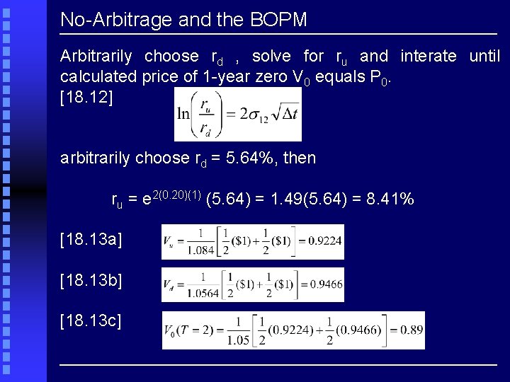
No-Arbitrage and the BOPM Arbitrarily choose rd , solve for ru and interate until calculated price of 1 -year zero V 0 equals P 0. [18. 12] arbitrarily choose rd = 5. 64%, then ru = e 2(0. 20)(1) (5. 64) = 1. 49(5. 64) = 8. 41% [18. 13 a] [18. 13 b] [18. 13 c]

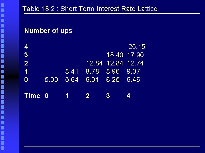
Table 18. 2 : Short Term Interest Rate Lattice Number of ups 4 3 2 1 0 5. 00 Time 0 8. 41 5. 64 25. 15 18. 40 17. 90 12. 84 12. 74 8. 78 8. 96 9. 07 6. 01 6. 25 6. 46 1 2 3 4

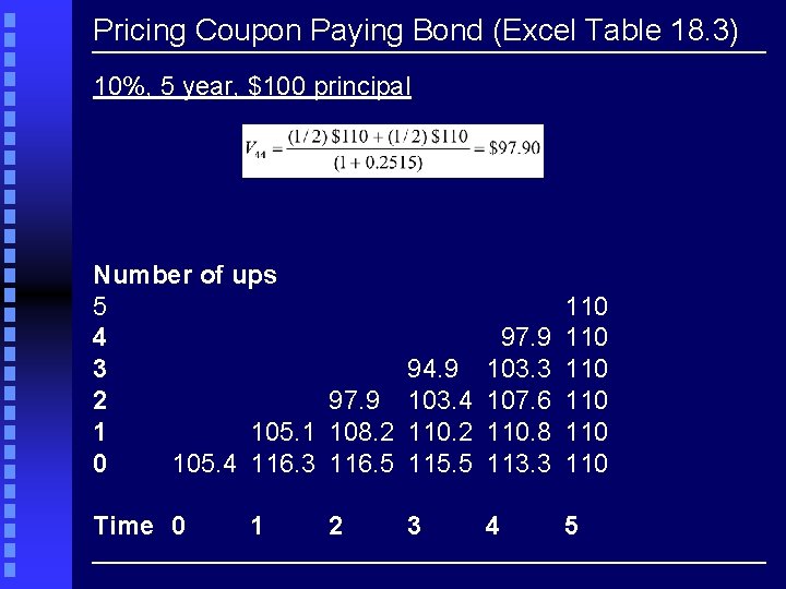
Pricing Coupon Paying Bond (Excel Table 18. 3) 10%, 5 year, $100 principal Number of ups 5 4 3 2 97. 9 1 105. 1 108. 2 0 105. 4 116. 3 116. 5 97. 9 94. 9 103. 3 103. 4 107. 6 110. 2 110. 8 115. 5 113. 3 110 110 110 Time 0 3 5 1 2 4

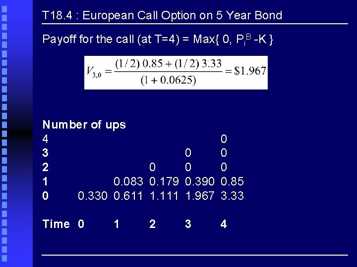
T 18. 4 : European Call Option on 5 Year Bond Payoff for the call (at T=4) = Max{ 0, Pi. B -K } Number of ups 4 3 2 0 1 0. 083 0. 179 0 0. 330 0. 611 1. 111 0 0 0. 390 0. 85 1. 967 3. 33 Time 0 3 1 2 4

T 18. 5: American Call on Coupon Bond

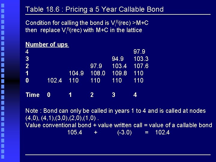
Table 18. 6 : Pricing a 5 Year Callable Bond Condition for calling the bond is Vi. B(rec) >M+C then replace Vi. B(rec) with M+C in the lattice Number of ups 4 3 2 1 104. 9 0 102. 4 110 Time 0 1 97. 9 108. 0 110 94. 9 103. 4 109. 8 110 97. 9 103. 3 107. 6 110 2 3 4 Note : Bond can only be called in years 1 to 4 and is called at nodes (4, 0), (4, 1), (3, 0), (2, 0), (1, 0). Value conventional bond + value written call = value of a callable bond 105. 4 + (-3. 0) = 102. 4

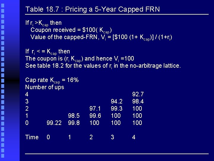
Table 18. 7 : Pricing a 5 -Year Capped FRN If ri >Kcap then Coupon received = $100( Kcap) Value of the capped-FRN, Vi = [$100 (1+ Kcap)] / (1+ri) If ri < = Kcap then The coupon is (ri Kcap) and hence Vi =100 See table 18. 2 for the values of ri in the no-arbitrage lattice. Cap rate Kcap = 16% Number of ups 4 3 2 1 98. 5 0 99. 22 99. 8 Time 0 1 97. 1 99. 6 100 94. 2 99. 3 100 92. 7 98. 4 100 100 2 3 4

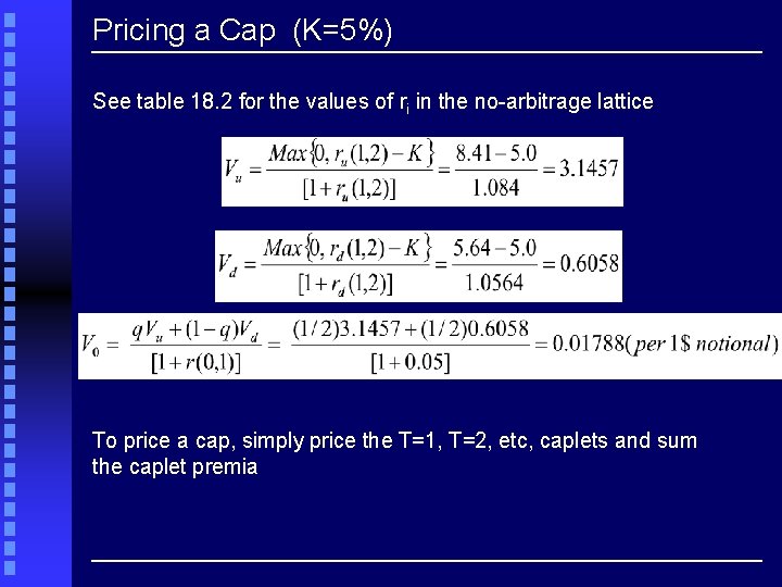
Pricing a Cap (K=5%) See table 18. 2 for the values of ri in the no-arbitrage lattice To price a cap, simply price the T=1, T=2, etc, caplets and sum the caplet premia

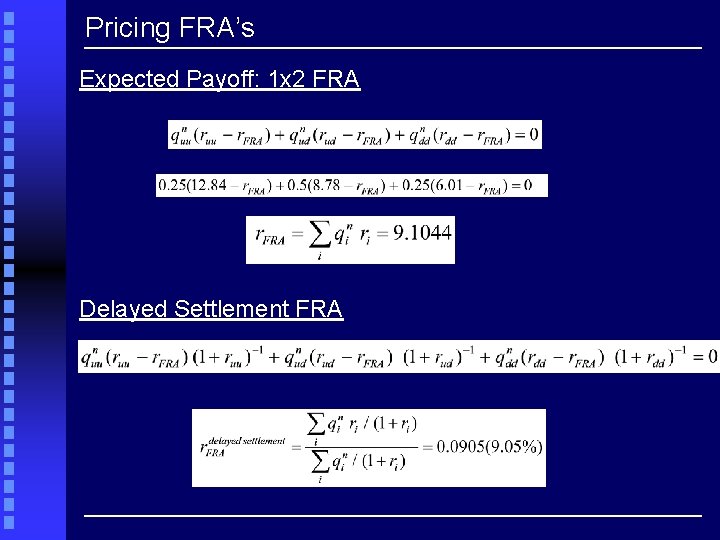
Pricing FRA’s Expected Payoff: 1 x 2 FRA Delayed Settlement FRA

MCS: Pricing a Caplet

MCS: Pricing a Caplet (Excel T 18. 10) Vasicek’s mean reverting model: [18. 53] rt – rt-1 = a ( b – rt-1 ) t + t Long run rate is b= 0. 08 (8%) Rate of convergence, ‘a’ = 0. 20 Current short rate is r 0 = 0. 10 (10%) Volatility, = 0. 007 Caplet Strike rate K= 0. 10 (10%) T = 1 year Divide 1 year into n=100 time units Take t = T/n = 0. 01

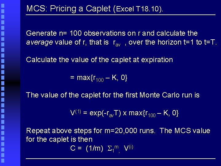
MCS: Pricing a Caplet (Excel T 18. 10). Generate n= 100 observations on r and calculate the average value of r, that is rav , over the horizon t=1 to t=T. Calculate the value of the caplet at expiration = max{r 100 – K, 0} The value of the caplet for the first Monte Carlo run is V(1) = exp(-rav. T) x max{r 100 – K, 0} Repeat above steps for m=20, 000 runs. The MCS value for the caplet is then C = (1/m) 1 m, V(i)

LECTURE ENDS HERE