Rational process models Tom Griffiths Department of Psychology

A strategy for studying the mind learning algorithm input output Determine the inductive biases

Marr’s three levels constrains Computation “What is the goal of the computation, why is

A problem learning algorithm input output

A problem learning algorithm input output How do inductive biases and representations in our

Relationship may not be transparent… • Assume people perform Bayesian inference, but with a

A simple demonstration • A causal learning task, where people form predictions and evaluate

Primes Strong Prime Teachers at an elementary school taught their students a game for

Phase 1 w m aa Consider what will happen if w and s touch.

Phase 2: Evaluating theories Please rate how good you find the following explanation: The

Results Phase 1 Phase 2 Estimated prior would depend on task (Bonawitz & Griffiths,

Why should we care? • This example shows we should be careful in the

A top-down approach… • The goal is approximating Bayesian inference • From computer science

The Monte Carlo principle where the x(i) are sampled from p(x)

Sampling as psychological process • Sampling can be done using existing “toolbox” – storage/retrieval,

Monte Carlo as mechanism • Importance sampling (Shi, Griffiths, Feldman, & Sanborn, 2010) •

Approximating Bayesian inference Sample from the prior, weight by the likelihood

Exemplar models • Assume decisions are made by storing previous events in memory, then

Equivalence Bayes can be approximated using exemplar models, storing hypotheses sampled from prior

Approximating Bayesian inference • Sample from prior, weight by likelihood • Can be implemented

The universal law of generalization (Shi, Griffiths, Feldman, & Sanborn, 2010)

The number game (Shi, Feldman, & Griffiths, 2008)

Making connections (Shi & Griffiths, 2009)

Win-stay, lose-shift algorithms • A class of algorithms that have been explored in both

Two interesting special cases • Case 1: Decide using only current likelihood • Case

Choice probabilities Go First No Go First (Bonawitz, Denison, Griffiths, & Gopnik, in press)

People Switch probabilities r = 0. 78 Win Stay, Lose Shift r = 0.

Updating distributions over time… • Computational costs are compounded when data are observed incrementally…

Particle filter weight by P(dn|h) samples from weighted atoms P(h|d 1, …, dn-1) P(h|d

Dynamic hypotheses h 1 h 2 h 3 h 4 d 1 d 2

Particle filters sample from P(h 4|h 3) weight by P(d 4|h 4) samples from

The promise of particle filters • A general scheme for defining rational process models

Simple garden-path sentences The woman brought the sandwich from the kitchen tripped

Particle filter with probabilistic grammars S NP VP 1. 0 V brought 0. 4

Simple garden-path sentences The woman brought the sandwich from the kitchen tripped MAIN VERB

Solving a puzzle A-S A-L U-S U-L Tom heard the gossip wasn’t true. Tom

Resampling-induced drift • In ambiguous region, observed words aren’t strongly informative • Due to

Markov chain Monte Carlo • Typically assumes all data are available, considers one hypothesis

Mechanistic pluralism Computation “What is the goal of the computation, why is it appropriate,

Conclusions • Bayesian models of cognition give us a way to identify human inductive

Slides: 56

Download presentation

Rational process models Tom Griffiths Department of Psychology Cognitive Science Program University of California, Berkeley

A strategy for studying the mind learning algorithm input output Determine the inductive biases of this human learning algorithm

Marr’s three levels constrains Computation “What is the goal of the computation, why is it appropriate, and what is the logic of the strategy by which it can be carried out? ” constrains Representation and algorithm “What is the representation for the input and output, and the algorithm for the transformation? ” Implementation “How can the representation and algorithm be realized physically? ”

A problem learning algorithm input output

A problem learning algorithm input output How do inductive biases and representations in our models connect to mental and neural processes?

Relationship may not be transparent… • Assume people perform Bayesian inference, but with a subset of all hypotheses – hypotheses are generated from a distribution q(h) • Behavior will still be consistent with Bayesian inference… • …but with a prior where h receives probability proportional to p(h)q(h) – the prior confounds two psychological factors: plausibility and ease of generation (Bonawitz & Griffiths, 2010)

A simple demonstration • A causal learning task, where people form predictions and evaluate explanations • Within-subjects, manipulate whether hypothesis generation is required – Phase 1: make predictions (requires generation) – Phase 2: provide all hypotheses, ask to evaluate • Between-subjects, manipulate ease of generation using a priming vignette – should only influence Phase 1 judgments (Bonawitz & Griffiths, 2010)

Primes Strong Prime Teachers at an elementary school taught their students a game for two children to play. They observed the results of pairs of students playing the game and tried to come up with a way to predict (for any given pair of students) who was going to win the game. At first it was difficult for the teachers to notice anything that would help them correctly predict the outcomes of the games. Then the teachers started organizing the children by the height of the children and the pattern of results quickly became apparent. The teachers were able to use the height of the children and make very accurate predictions as to who (for any given pair of students) was going to win the game. Neutral Prime Teachers at an elementary school taught their students a game for two children to play. They observed the results of pairs of students playing the game and tried to come up with a way to predict (for any given pair of students) who was going to win the game. At first it was difficult for the teachers to notice anything that would help them correctly predict the outcomes of the games. Then the teachers started organizing the children by the children’s shirt color and the pattern of results quickly became apparent. The teachers were able to use the color of the children’s shirts and make very accurate predictions as to who (for any given pair of students) was going to win the game. (Bonawitz & Griffiths, 2010)

Phase 1 w m aa Consider what will happen if w and s touch. Will w light? Yes No How confident are you? 1 2 3 4 5 6 7 Not sure Very Sure Will s light? Yes No How confident are you? 1 2 3 4 5 6 7 Not sure Very Sure The blocks are slid together and, m Consider what will happen if w and k touch. w Will w light? Yes No How confident are you? 1 2 3 4 5 6 7 Block w lights up! Also observed so far: m y k s y s Not sure Very Sure Will k light? Yes No How confident are you? 1 2 3 4 5 6 7 Not sure Very Sure

Phase 2: Evaluating theories Please rate how good you find the following explanation: The blocks can not be organized. They will light or not light randomly, but only one block can be lit at a time. The blocks can be organized by ‘strength’. The stronger blocks will light the weaker ones: Strongest s k 1 2 3 Not good 4 5 6 7 Very good 1 2 3 Not good m y 4 5 Weakest w/g 6 7 Very good

Results Phase 1 Phase 2 Estimated prior would depend on task (Bonawitz & Griffiths, 2010)

Why should we care? • This example shows we should be careful in the psychological interpretation of priors • We should be similarly careful in the psychological interpretation of representations • The only way to understand how computational level models constrain algorithmic level models is to begin to connect the two…

A top-down approach… • The goal is approximating Bayesian inference • From computer science and statistics, find good methods for solving this problem • See if these methods can be connected to psychological processes • The result: “rational process models” (Sanborn et al. , 2006; Shi et al. , 2008)

The Monte Carlo principle where the x(i) are sampled from p(x)

Sampling as psychological process • Sampling can be done using existing “toolbox” – storage/retrieval, simulation, activation/competition • Many existing process models use sampling: – Luce choice rule (Luce, 1959) – stochastic models of reaction time – used to explain correlation perception, confidence intervals, utility curves, … (Kareev, 2000; Fiedler & Juslin, 2006; Stewart et al. , 2006)

Monte Carlo as mechanism • Importance sampling (Shi, Griffiths, Feldman, & Sanborn, 2010) • “Win-stay, lose-shift” algorithms (Bonawitz, Denison, Griffiths, & Gopnik, in press) • Particle filters (Brown & Steyvers, 2009; Daw & Courville, 2008; Levy et al. , 2009; Sanborn et al. , 2010) • Markov chain Monte Carlo (Gershman, Vul, & Tenenbaum, 2009; Ullman, Goodman, & Tenenbaum, 2010)

Importance sampling q(x) p(x)

Approximating Bayesian inference Sample from the prior, weight by the likelihood

Exemplar models • Assume decisions are made by storing previous events in memory, then activating by similarity • For example, categorization: where x(i) are exemplars, s(x, x(i)) is similarity, I(x(i) c) is 1 if x(i) is from category c (e. g. , Nosofsky, 1986)

Exemplar models • Assume decisions are made by storing previous events in memory, then activating by similarity • General version: where x(i) are exemplars, s(x, x(i)) is similarity, f(x(i)) is quantity of interest

Equivalence Bayes can be approximated using exemplar models, storing hypotheses sampled from prior

Approximating Bayesian inference • Sample from prior, weight by likelihood • Can be implemented in an exemplar model – store “exemplars” of hypotheses through experience – activate in proportion to likelihood (=“similarity”) (Shi, Feldman, & Griffiths, 2008)

The universal law of generalization (Shi, Griffiths, Feldman, & Sanborn, 2010)

The number game (Shi, Feldman, & Griffiths, 2008)

Making connections (Shi & Griffiths, 2009)

Win-stay, lose-shift algorithms • A class of algorithms that have been explored in both computer science and psychology • Our version: After observing dn, keep hypothesis h with probability where c can depend on d 1, …dn-1, and is such that [0, 1] else sample h from P(h|d 1, …, dn) • Then h is a sample from P(h|d 1, …, dn) for all n (Bonawitz, Denison, Griffiths, & Gopnik, in press)

Two interesting special cases • Case 1: Decide using only current likelihood • Case 2 : Minimize the rate of switching (Bonawitz, Denison, Griffiths, & Gopnik, in press)

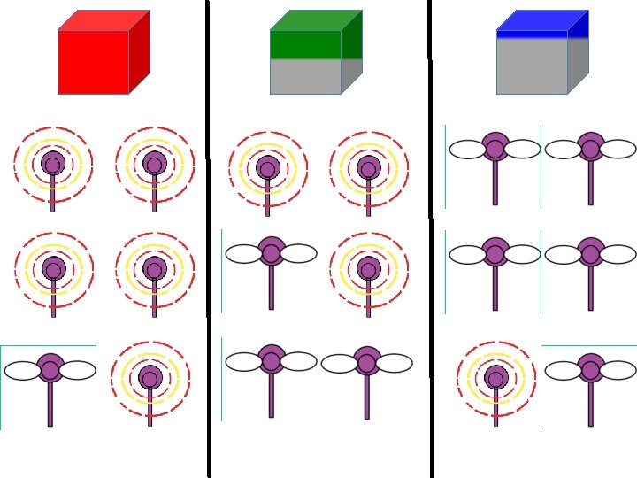
Blicket Detector

Go First No Go First:

Choice probabilities Go First No Go First (Bonawitz, Denison, Griffiths, & Gopnik, in press)

People Switch probabilities r = 0. 78 Win Stay, Lose Shift r = 0. 38 Independent sampling (Bonawitz, Denison, Griffiths, & Gopnik, in press)

Monte Carlo as mechanism • Importance sampling (Shi, Griffiths, Feldman, & Sanborn, 2010) • “Win-stay, lose-shift” algorithms (Bonawitz, Denison, Griffiths, & Gopnik, in press) • Particle filters (Brown & Steyvers, 2009; Daw & Courville, 2008; Levy et al. , 2009; Sanborn et al. , 2010; ) • Markov chain Monte Carlo (Gershman, Vul, & Tenenbaum, 2009; Ullman, Goodman, & Tenenbaum, 2010)

Updating distributions over time… • Computational costs are compounded when data are observed incrementally… – recompute P(h|d 1, …, dn) after observing dn • Exploit “yesterday’s posterior is today’s prior” • Repeatedly using importance sampling results in an algorithm known as a “particle filter”

Particle filter weight by P(dn|h) samples from weighted atoms P(h|d 1, …, dn-1) P(h|d 1, …, dn) samples from P(h|d 1, …, dn)

Dynamic hypotheses h 1 h 2 h 3 h 4 d 1 d 2 d 3 d 4

The promise of particle filters • A general scheme for defining rational process models of updating over time (Sanborn et al. , 2006) • Model limited memory, and produce order effects (cf. Kruschke, 2006) • Used to define rational process models of… – categorization – associative learning – changepoint detection – sentence processing (Sanborn et al. , 2006) (Daw & Courville, 2008) (Brown & Steyvers, 2009) (Levy et a 1. , 2009)

Simple garden-path sentences The woman brought the sandwich from the kitchen tripped

Particle filter with probabilistic grammars S NP VP 1. 0 V brought 0. 4 NP N 0. 8 V broke 0. 3 NP N RRC 0. 2 V tripped 0. 3 RRC Part N 1. 0 Part brought 0. 1 VP VN 1. 0 Part broken 0. 7 N woman 0. 7 Part tripped 0. 2 N sandwiches 0. 3 Adv quickly 1. 0 S * NP* * N* * VP * RRC* * Part* * woman brought 0. 7 0. 1 N * * V* * sandwiches tripped 0. 3

Simple garden-path sentences The woman brought the sandwich from the kitchen tripped MAIN VERB (it was the woman who brought the sandwich) REDUCED RELATIVE (the woman was brought the sandwich)

Solving a puzzle A-S A-L U-S U-L Tom heard the gossip wasn’t true. Tom heard the gossip about the neighbors wasn’t true. Tom heard that the gossip about the neighbors wasn’t true. • Ambiguity increases difficulty… • …but so does the length of the ambiguous region (Frazier & Rayner, 1982; Tabor & Hutchins, 2004) • Our prediction: parse failures at the disambiguating region should increase with sentence difficulty

Resampling-induced drift • In ambiguous region, observed words aren’t strongly informative • Due to resampling, probabilities of different constructions will drift (more so with time)

Model results

Markov chain Monte Carlo • Typically assumes all data are available, considers one hypothesis at a time and stochastically explores the space of hypotheses • A possible account of perceptual bistability (Gershman, Vul, & Tenenbaum, 2009) • A way to explain how children explore the space of possible causal theories (Ullman, Goodman, & Tenenbaum, 2010)

Mechanistic pluralism Computation “What is the goal of the computation, why is it appropriate, and what is the logic of the strategy by which it can be carried out? ” Representation and algorithm … “What is the. WSLS representation for the input and output, Importance Particle MCMC sampling filtering and the algorithm for the transformation? ” Implementation “How can Associative the representation and algorithm be Probabilistic RBF coding realized physically? ” networks memories …

Conclusions • Bayesian models of cognition give us a way to identify human inductive biases • But, the relationship of priors and representations in these models to mental and neural processes is not necessarily transparent • Monte Carlo methods provide a source of rational process models that could connect these levels, and perhaps the expectation of many mechanisms