3 6 Rational Functions Rational Functions A rational

3. 6 Rational Functions

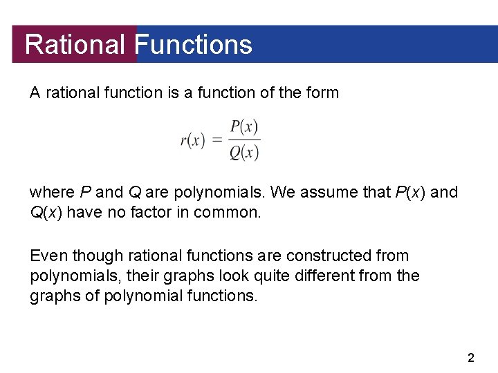
Rational Functions A rational function is a function of the form where P and Q are polynomials. We assume that P(x) and Q(x) have no factor in common. Even though rational functions are constructed from polynomials, their graphs look quite different from the graphs of polynomial functions. 2

Rational Functions and Asymptotes The domain of a rational function consists of all real numbers x except those for which the denominator is zero. When graphing a rational function, we must pay special attention to the behavior of the graph near those x-values. We begin by graphing a very simple rational function. 3

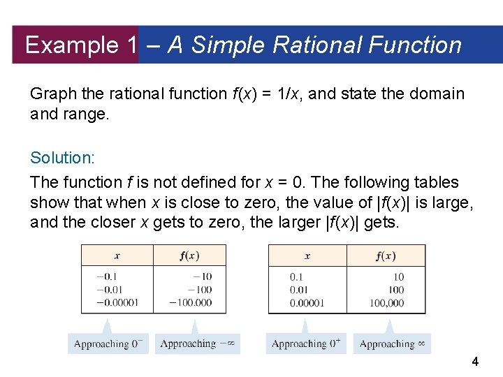
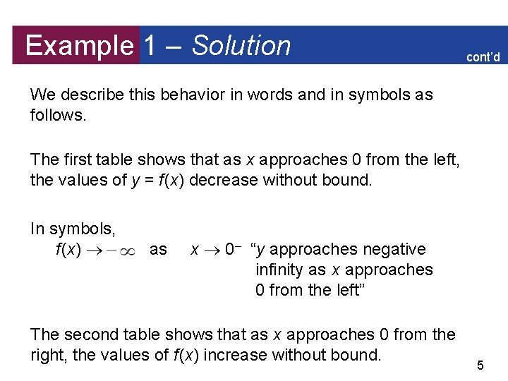
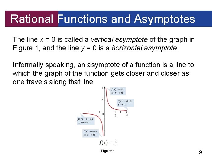
Example 1 – A Simple Rational Function Graph the rational function f (x) = 1/x, and state the domain and range. Solution: The function f is not defined for x = 0. The following tables show that when x is close to zero, the value of |f (x)| is large, and the closer x gets to zero, the larger |f (x)| gets. 4

Example 1 – Solution cont’d We describe this behavior in words and in symbols as follows. The first table shows that as x approaches 0 from the left, the values of y = f (x) decrease without bound. In symbols, f (x) as x 0– “y approaches negative infinity as x approaches 0 from the left” The second table shows that as x approaches 0 from the right, the values of f (x) increase without bound. 5

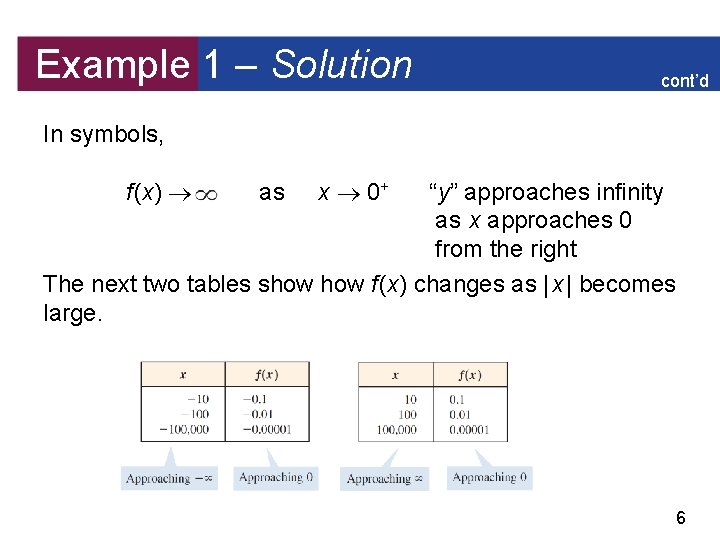
Example 1 – Solution cont’d In symbols, f (x) as x 0+ “y” approaches infinity as x approaches 0 from the right The next two tables show f (x) changes as | x | becomes large. 6

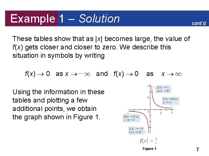
Example 1 – Solution cont’d These tables show that as |x| becomes large, the value of f (x) gets closer and closer to zero. We describe this situation in symbols by writing f (x) 0 as x and f (x) 0 as x Using the information in these tables and plotting a few additional points, we obtain the graph shown in Figure 1 7

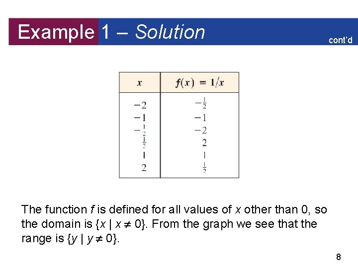
Example 1 – Solution cont’d The function f is defined for all values of x other than 0, so the domain is {x | x 0}. From the graph we see that the range is {y | y 0}. 8

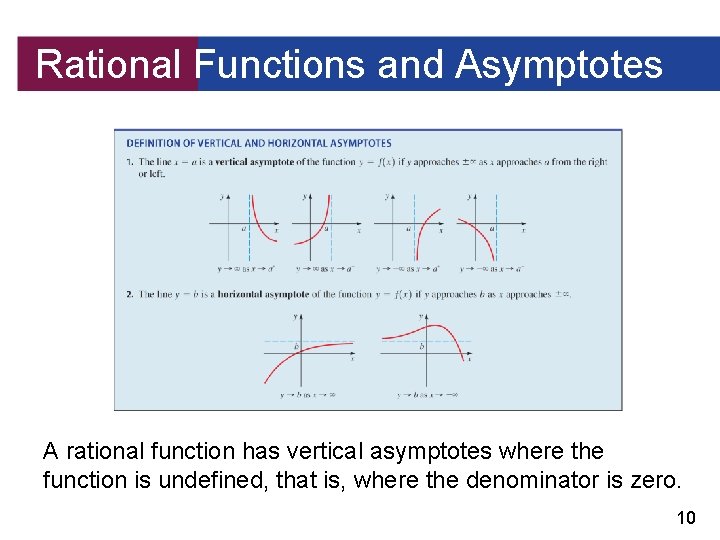
Rational Functions and Asymptotes The line x = 0 is called a vertical asymptote of the graph in Figure 1, and the line y = 0 is a horizontal asymptote. Informally speaking, an asymptote of a function is a line to which the graph of the function gets closer and closer as one travels along that line. Figure 1 9

Rational Functions and Asymptotes A rational function has vertical asymptotes where the function is undefined, that is, where the denominator is zero. 10

Transformations of y = 1/x 11

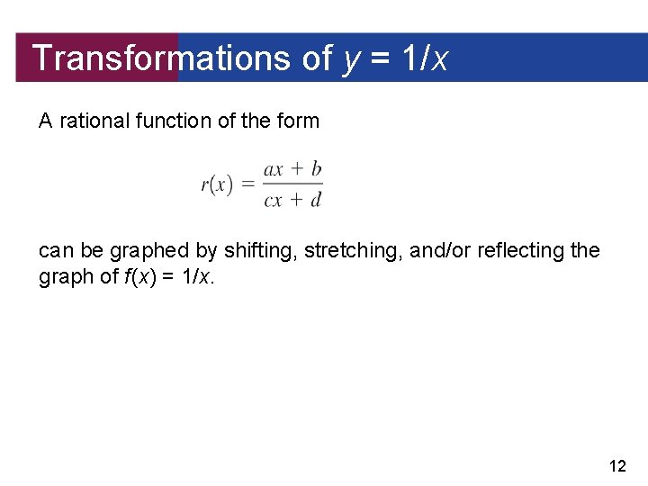
Transformations of y = 1/x A rational function of the form can be graphed by shifting, stretching, and/or reflecting the graph of f (x) = 1/x. 12

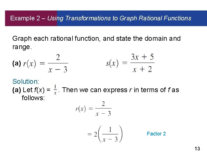
Example 2 – Using Transformations to Graph Rational Functions Graph each rational function, and state the domain and range. (a) (b) Solution: (a) Let f (x) = follows: . Then we can express r in terms of f as Factor 2 13

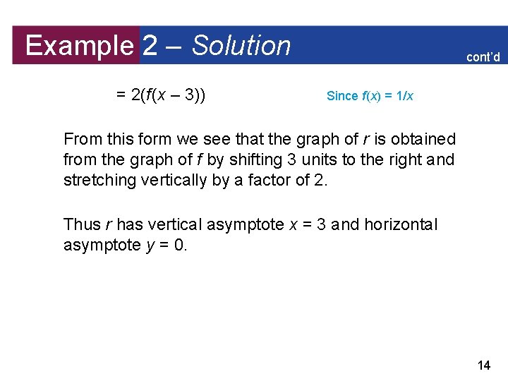
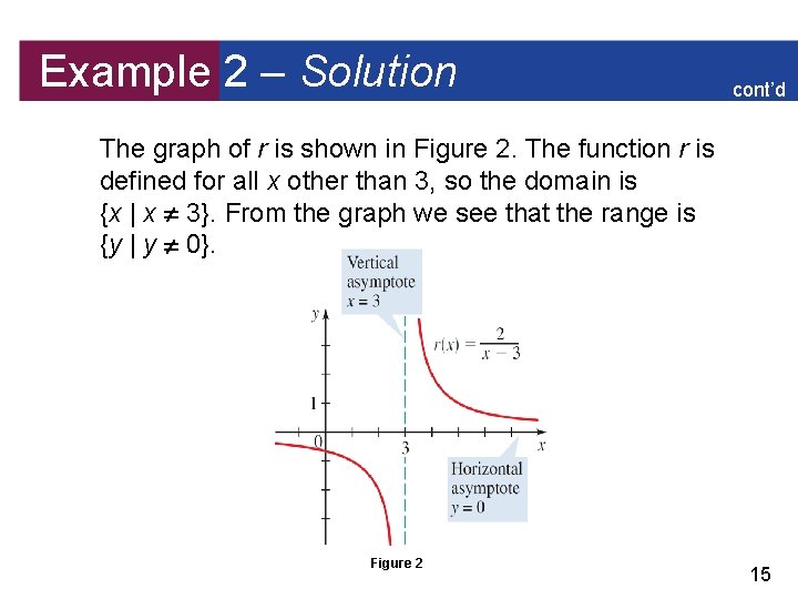
Example 2 – Solution = 2(f (x – 3)) cont’d Since f (x) = 1/x From this form we see that the graph of r is obtained from the graph of f by shifting 3 units to the right and stretching vertically by a factor of 2. Thus r has vertical asymptote x = 3 and horizontal asymptote y = 0. 14

Example 2 – Solution cont’d The graph of r is shown in Figure 2. The function r is defined for all x other than 3, so the domain is {x | x 3}. From the graph we see that the range is {y | y 0}. Figure 2 15

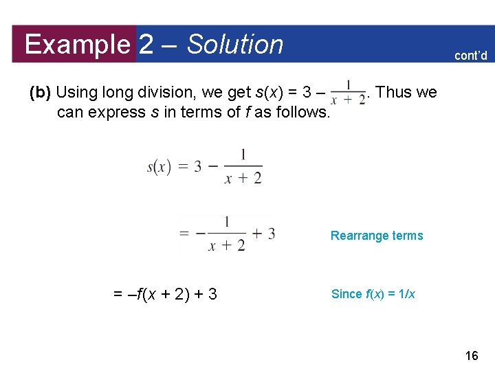
Example 2 – Solution cont’d (b) Using long division, we get s (x) = 3 – can express s in terms of f as follows. . Thus we Rearrange terms = –f (x + 2) + 3 Since f (x) = 1/x 16

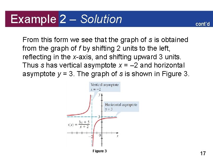
Example 2 – Solution cont’d From this form we see that the graph of s is obtained from the graph of f by shifting 2 units to the left, reflecting in the x-axis, and shifting upward 3 units. Thus s has vertical asymptote x = – 2 and horizontal asymptote y = 3. The graph of s is shown in Figure 3 17

Example 2 – Solution cont’d The function s is defined for all x other than – 2, so the domain is {x | x – 2}. From the graph we see that the range is {y | y 3}. 18

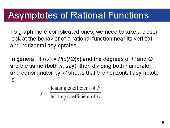
Asymptotes of Rational Functions To graph more complicated ones, we need to take a closer look at the behavior of a rational function near its vertical and horizontal asymptotes. In general, if r (x) = P(x)/Q(x) and the degrees of P and Q are the same (both n, say), then dividing both numerator and denominator by xn shows that the horizontal asymptote is 19

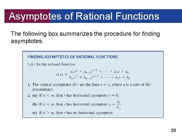
Asymptotes of Rational Functions The following box summarizes the procedure for finding asymptotes. 20

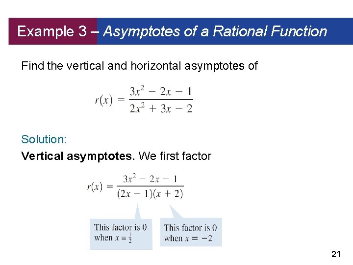
Example 3 – Asymptotes of a Rational Function Find the vertical and horizontal asymptotes of Solution: Vertical asymptotes. We first factor 21

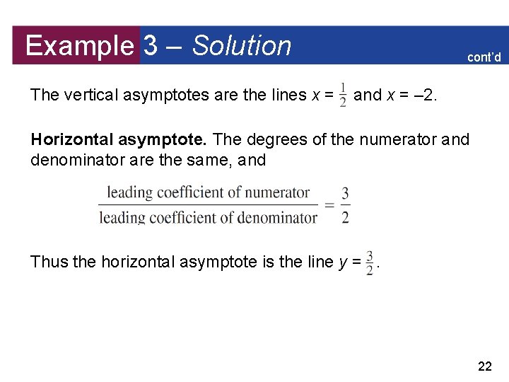
Example 3 – Solution The vertical asymptotes are the lines x = cont’d and x = – 2. Horizontal asymptote. The degrees of the numerator and denominator are the same, and Thus the horizontal asymptote is the line y =. 22

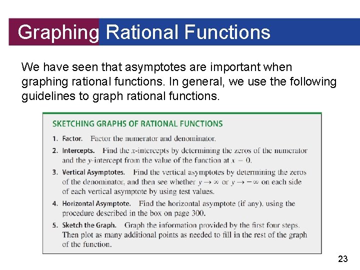
Graphing Rational Functions We have seen that asymptotes are important when graphing rational functions. In general, we use the following guidelines to graph rational functions. 23

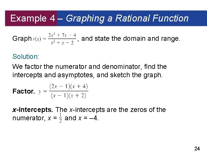
Example 4 – Graphing a Rational Function Graph , and state the domain and range. Solution: We factor the numerator and denominator, find the intercepts and asymptotes, and sketch the graph. Factor. x-Intercepts. The x-intercepts are the zeros of the numerator, x = and x = – 4. 24

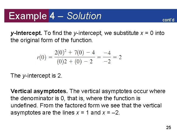
Example 4 – Solution cont’d y-Intercept. To find the y-intercept, we substitute x = 0 into the original form of the function. The y-intercept is 2. Vertical asymptotes. The vertical asymptotes occur where the denominator is 0, that is, where the function is undefined. From the factored form we see that the vertical asymptotes are the lines x = 1 and x = – 2. 25

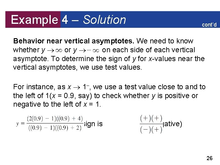
Example 4 – Solution cont’d Behavior near vertical asymptotes. We need to know whether y on each side of each vertical asymptote. To determine the sign of y for x-values near the vertical asymptotes, we use test values. For instance, as x 1–, we use a test value close to and to the left of 1(x = 0. 9, say) to check whether y is positive or negative to the left of x = 1. whose sign is (negative) 26

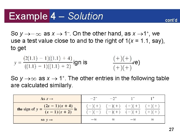
Example 4 – Solution cont’d So y as x 1–. On the other hand, as x 1+, we use a test value close to and to the right of 1(x = 1. 1, say), to get whose sign is (positive) So y as x 1+. The other entries in the following table are calculated similarly. 27

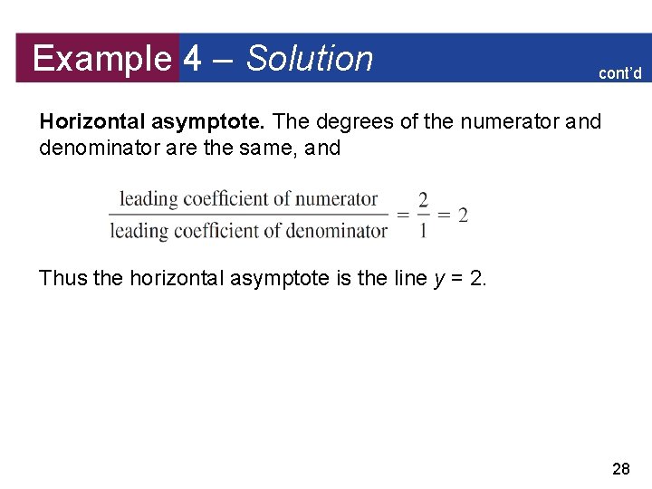
Example 4 – Solution cont’d Horizontal asymptote. The degrees of the numerator and denominator are the same, and Thus the horizontal asymptote is the line y = 2. 28

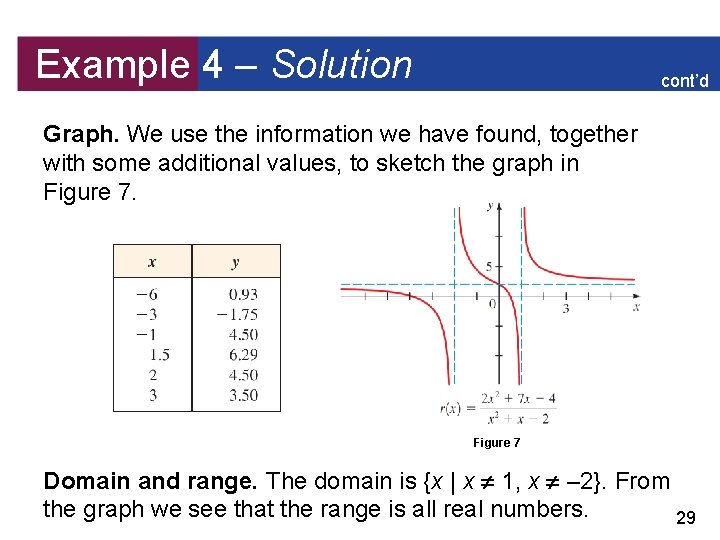
Example 4 – Solution cont’d Graph. We use the information we have found, together with some additional values, to sketch the graph in Figure 7 Domain and range. The domain is {x | x 1, x – 2}. From the graph we see that the range is all real numbers. 29

Common Factors in Numerator and Denominator We have adopted the convention that the numerator and denominator of a rational function have no factor in common. If s(x) = p(x)/q(x) and if p and q do have a factor in common, then we may cancel that factor, but only for those values of x for which that factor is not zero (because division by zero is not defined). Since s is not defined at those values of x, its graph has a “hole” at those points. 30

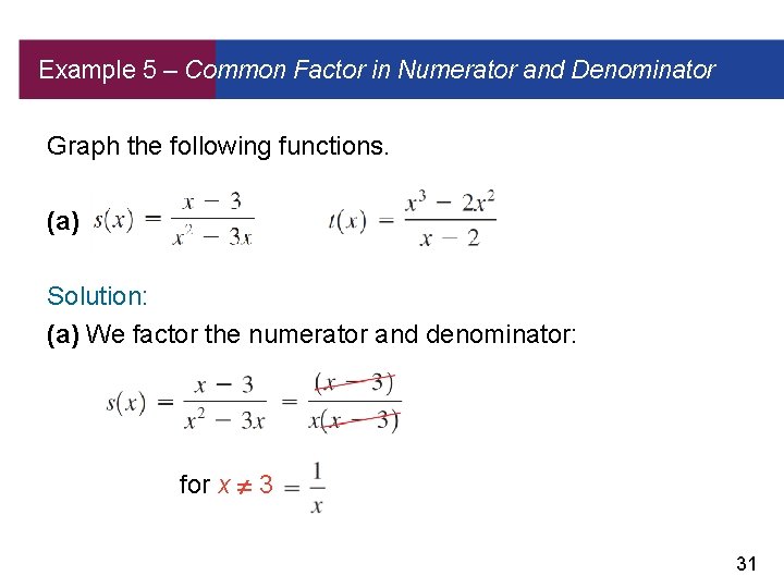
Example 5 – Common Factor in Numerator and Denominator Graph the following functions. (a) (b) Solution: (a) We factor the numerator and denominator: for x 3 31

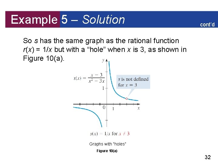
Example 5 – Solution cont’d So s has the same graph as the rational function r(x) = 1/x but with a “hole” when x is 3, as shown in Figure 10(a). Graphs with “holes” Figure 10(a) 32

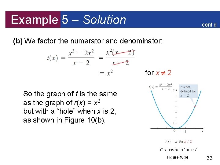
Example 5 – Solution cont’d (b) We factor the numerator and denominator: for x 2 So the graph of t is the same as the graph of r(x) = x 2 but with a “hole” when x is 2, as shown in Figure 10(b). Graphs with “holes” Figure 10(b) 33

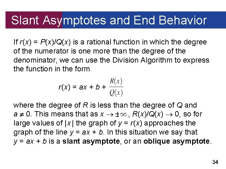
Slant Asymptotes and End Behavior If r (x) = P(x)/Q(x) is a rational function in which the degree of the numerator is one more than the degree of the denominator, we can use the Division Algorithm to express the function in the form r (x) = ax + b + where the degree of R is less than the degree of Q and a 0. This means that as x , R(x)/Q(x) 0, so for large values of | x | the graph of y = r (x) approaches the graph of the line y = ax + b. In this situation we say that y = ax + b is a slant asymptote, or an oblique asymptote. 34

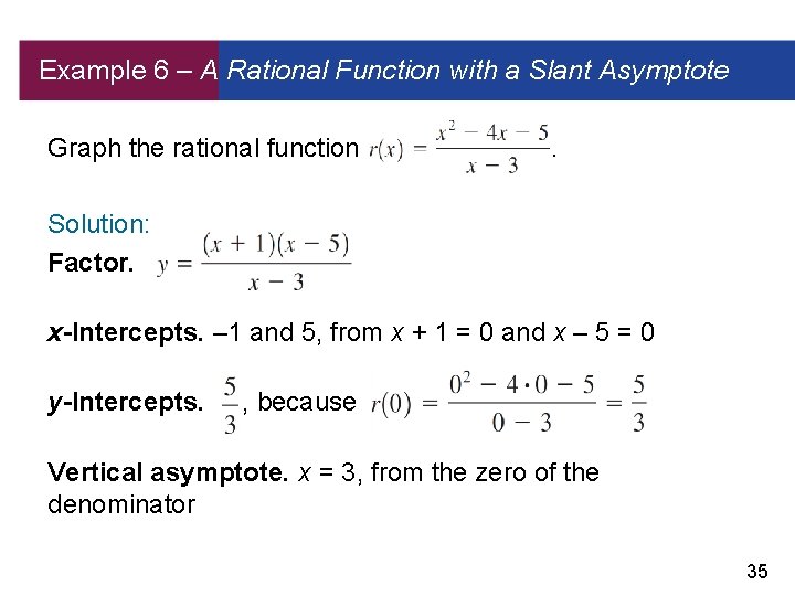
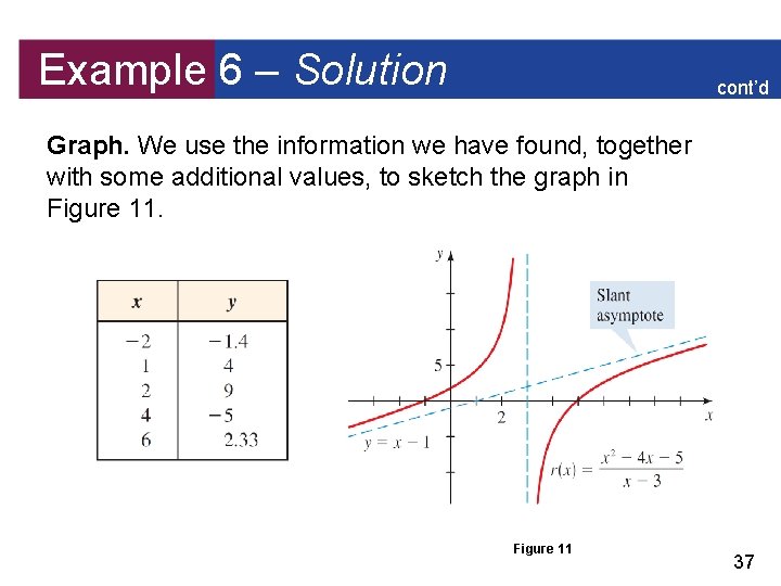
Example 6 – A Rational Function with a Slant Asymptote Graph the rational function . Solution: Factor. x-Intercepts. – 1 and 5, from x + 1 = 0 and x – 5 = 0 y-Intercepts. , because Vertical asymptote. x = 3, from the zero of the denominator 35

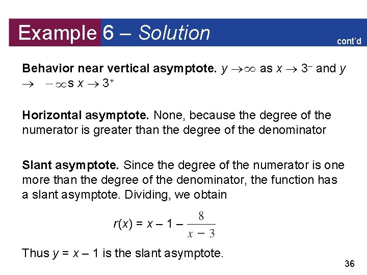
Example 6 – Solution Behavior near vertical asymptote. y as x 3+ cont’d as x 3– and y Horizontal asymptote. None, because the degree of the numerator is greater than the degree of the denominator Slant asymptote. Since the degree of the numerator is one more than the degree of the denominator, the function has a slant asymptote. Dividing, we obtain r (x) = x – 1 – Thus y = x – 1 is the slant asymptote. 36

Example 6 – Solution cont’d Graph. We use the information we have found, together with some additional values, to sketch the graph in Figure 11 37

Applications Rational functions occur frequently in scientific applications of algebra. In the next example we analyze the graph of a function from theory of electricity. 38

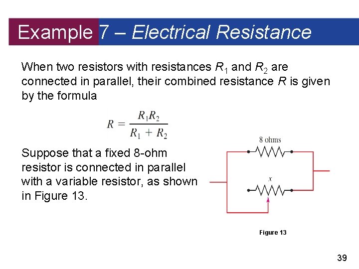
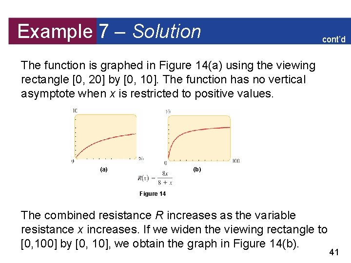
Example 7 – Electrical Resistance When two resistors with resistances R 1 and R 2 are connected in parallel, their combined resistance R is given by the formula Suppose that a fixed 8 -ohm resistor is connected in parallel with a variable resistor, as shown in Figure 13 39

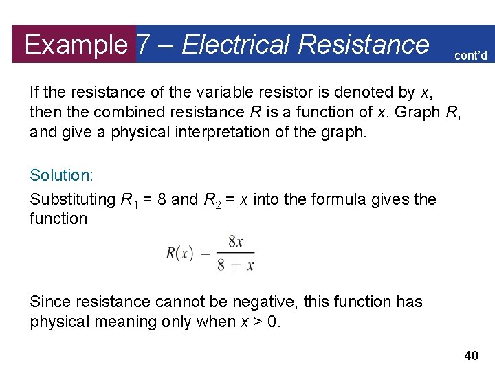
Example 7 – Electrical Resistance cont’d If the resistance of the variable resistor is denoted by x, then the combined resistance R is a function of x. Graph R, and give a physical interpretation of the graph. Solution: Substituting R 1 = 8 and R 2 = x into the formula gives the function Since resistance cannot be negative, this function has physical meaning only when x > 0. 40

Example 7 – Solution cont’d The function is graphed in Figure 14(a) using the viewing rectangle [0, 20] by [0, 10]. The function has no vertical asymptote when x is restricted to positive values. (a) (b) Figure 14 The combined resistance R increases as the variable resistance x increases. If we widen the viewing rectangle to [0, 100] by [0, 10], we obtain the graph in Figure 14(b). 41

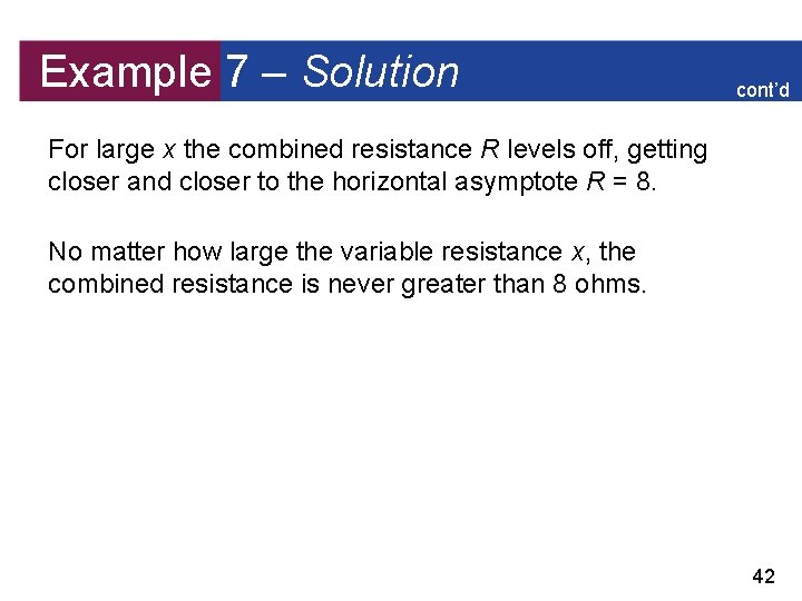
Example 7 – Solution cont’d For large x the combined resistance R levels off, getting closer and closer to the horizontal asymptote R = 8. No matter how large the variable resistance x, the combined resistance is never greater than 8 ohms. 42

3. 7 Polynomial and Rational Inequalities 43

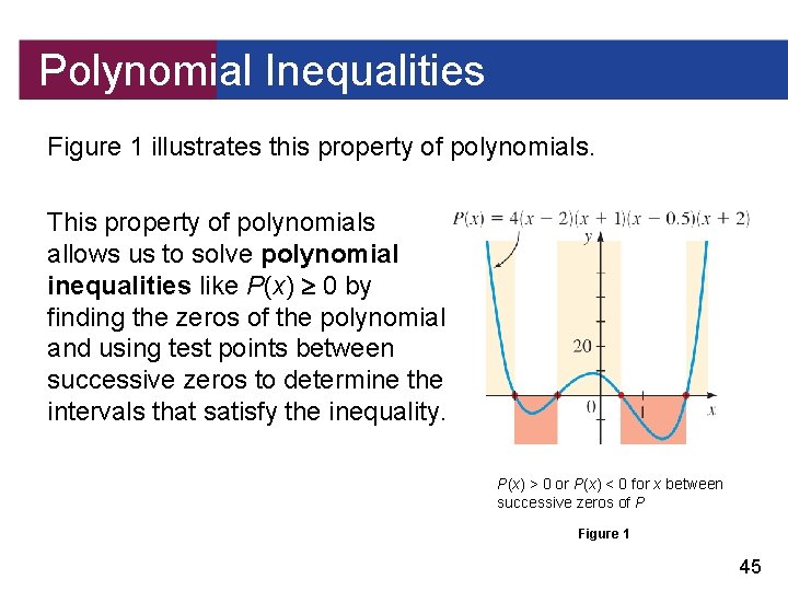
Polynomial Inequalities An important consequence of the Intermediate Value Theorem is that the values of a polynomial function P do not change sign between successive zeros. In other words, the values of P between successive zeros are either all positive or all negative. Graphically, this means that between successive x-intercepts, the graph of P is entirely above or entirely below the x-axis. 44

Polynomial Inequalities Figure 1 illustrates this property of polynomials. This property of polynomials allows us to solve polynomial inequalities like P(x) 0 by finding the zeros of the polynomial and using test points between successive zeros to determine the intervals that satisfy the inequality. P(x) > 0 or P(x) < 0 for x between successive zeros of P Figure 1 45

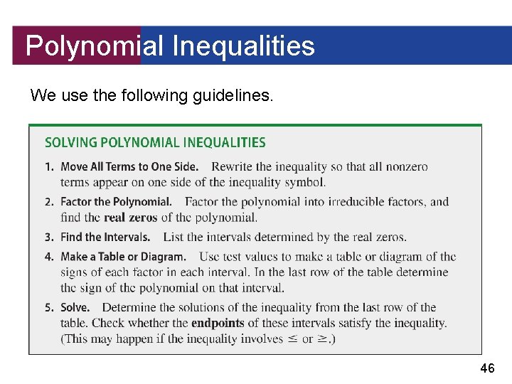
Polynomial Inequalities We use the following guidelines. 46

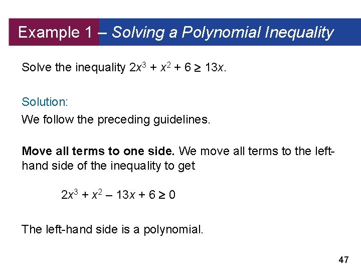
Example 1 – Solving a Polynomial Inequality Solve the inequality 2 x 3 + x 2 + 6 13 x. Solution: We follow the preceding guidelines. Move all terms to one side. We move all terms to the lefthand side of the inequality to get 2 x 3 + x 2 – 13 x + 6 0 The left-hand side is a polynomial. 47

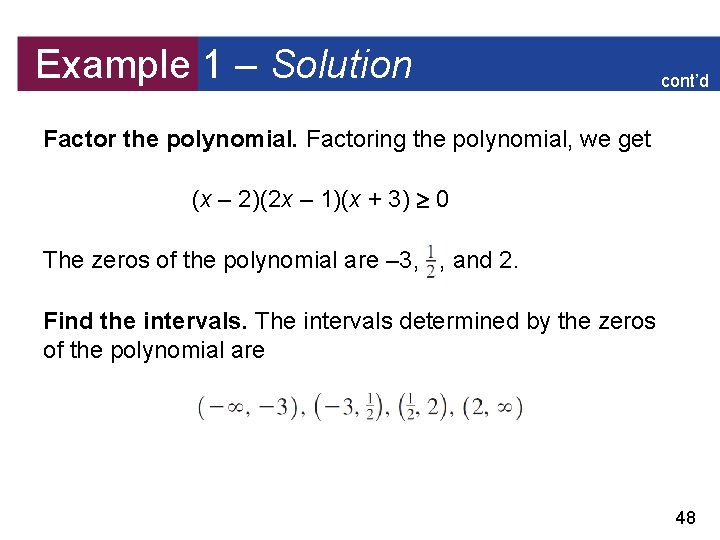
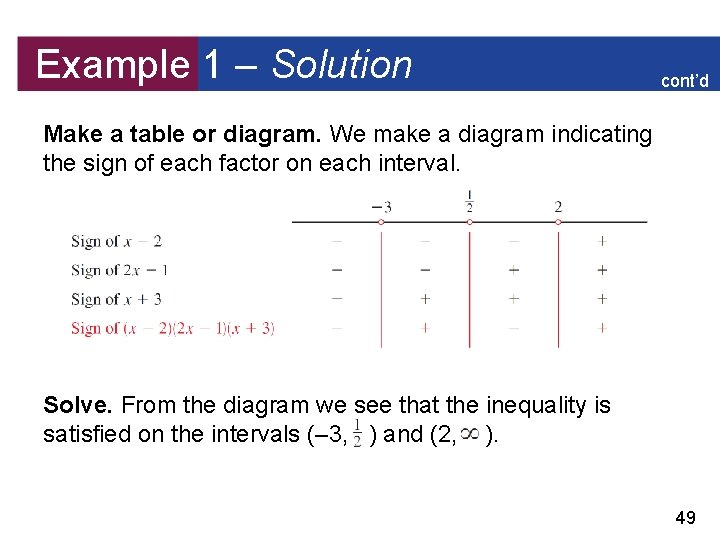
Example 1 – Solution cont’d Factor the polynomial. Factoring the polynomial, we get (x – 2)(2 x – 1)(x + 3) 0 The zeros of the polynomial are – 3, , and 2. Find the intervals. The intervals determined by the zeros of the polynomial are 48

Example 1 – Solution cont’d Make a table or diagram. We make a diagram indicating the sign of each factor on each interval. Solve. From the diagram we see that the inequality is satisfied on the intervals (– 3, ) and (2, ). 49

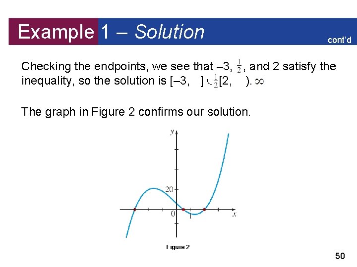
Example 1 – Solution cont’d Checking the endpoints, we see that – 3, , and 2 satisfy the inequality, so the solution is [– 3, ] [2, ). The graph in Figure 2 confirms our solution. Figure 2 50

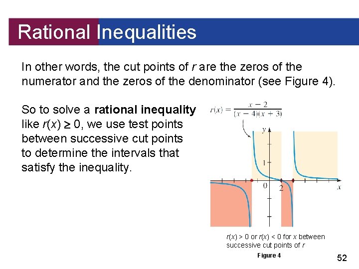
Rational Inequalities Unlike polynomial functions, rational functions are not necessarily continuous. The vertical asymptotes of a rational function r break up the graph into separate “branches. ” So the intervals on which r does not change sign are determined by the vertical asymptotes as well as the zeros of r. This is the reason for the following definition: If r(x) = P(x)/Q(x) is a rational function, the cut points of r are the values of x at which either P(x) = 0 or Q(x) = 0. 51

Rational Inequalities In other words, the cut points of r are the zeros of the numerator and the zeros of the denominator (see Figure 4). So to solve a rational inequality like r(x) 0, we use test points between successive cut points to determine the intervals that satisfy the inequality. r(x) > 0 or r(x) < 0 for x between successive cut points of r Figure 4 52

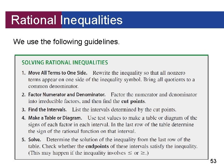
Rational Inequalities We use the following guidelines. 53

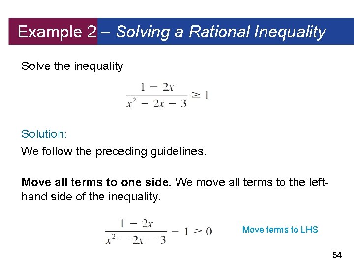
Example 2 – Solving a Rational Inequality Solve the inequality Solution: We follow the preceding guidelines. Move all terms to one side. We move all terms to the lefthand side of the inequality. Move terms to LHS 54

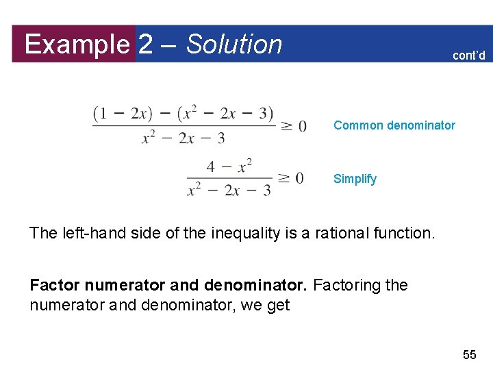
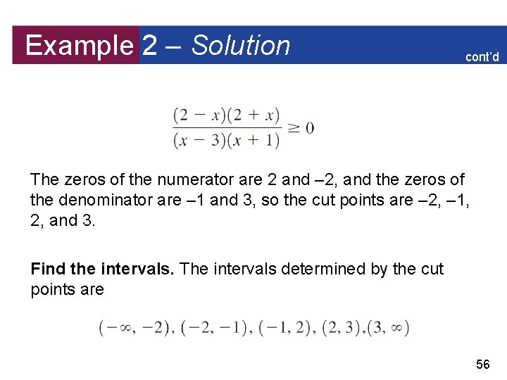
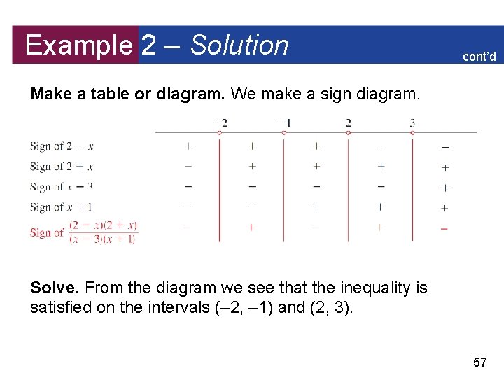
Example 2 – Solution cont’d Common denominator Simplify The left-hand side of the inequality is a rational function. Factor numerator and denominator. Factoring the numerator and denominator, we get 55

Example 2 – Solution cont’d The zeros of the numerator are 2 and – 2, and the zeros of the denominator are – 1 and 3, so the cut points are – 2, – 1, 2, and 3. Find the intervals. The intervals determined by the cut points are 56

Example 2 – Solution cont’d Make a table or diagram. We make a sign diagram. Solve. From the diagram we see that the inequality is satisfied on the intervals (– 2, – 1) and (2, 3). 57

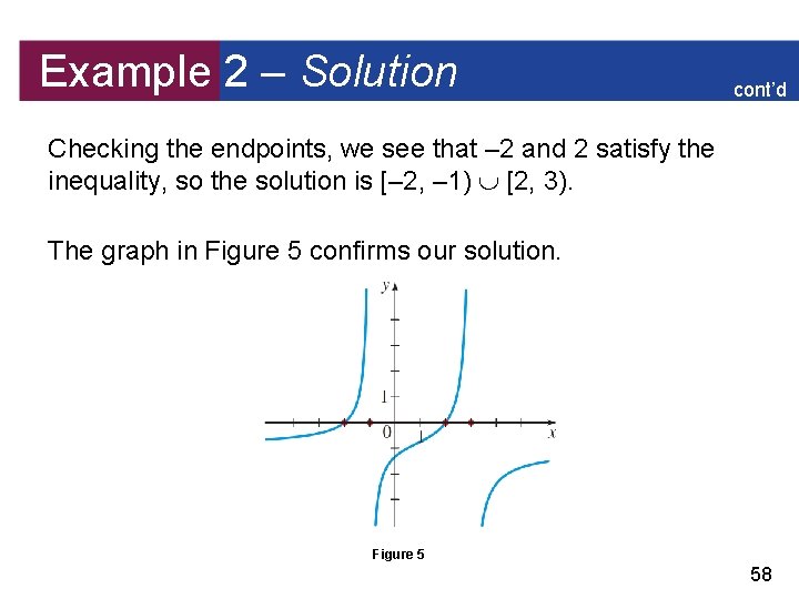
Example 2 – Solution cont’d Checking the endpoints, we see that – 2 and 2 satisfy the inequality, so the solution is [– 2, – 1) [2, 3). The graph in Figure 5 confirms our solution. Figure 5 58