Principal Component Analysis and Linear Discriminant Analysis ChaurChin

Principal Component Analysis and Linear Discriminant Analysis Chaur-Chin Chen Institute of Information Systems and Applications National Tsing Hua University Hsinchu 30013, Taiwan E-mail: cchen@cs. nthu. edu. tw

Outline ◇ Motivation for PCA ◇ Problem Statement for PCA ◇ The Solution and Practical Computations ◇ Examples and Undesired Results ◇ Fundamentals of LDA ◇ Discriminant Analysis ◇ Practical Computations ◇ Examples and Comparison with PCA

Motivation ß ß Principal Component Analysis (PCA) and Linear Discriminant Analysis (LDA) are multivariate statistical techniques that are often useful in reducing dimensionality of a collection of unstructured random variables for analysis and interpretation.

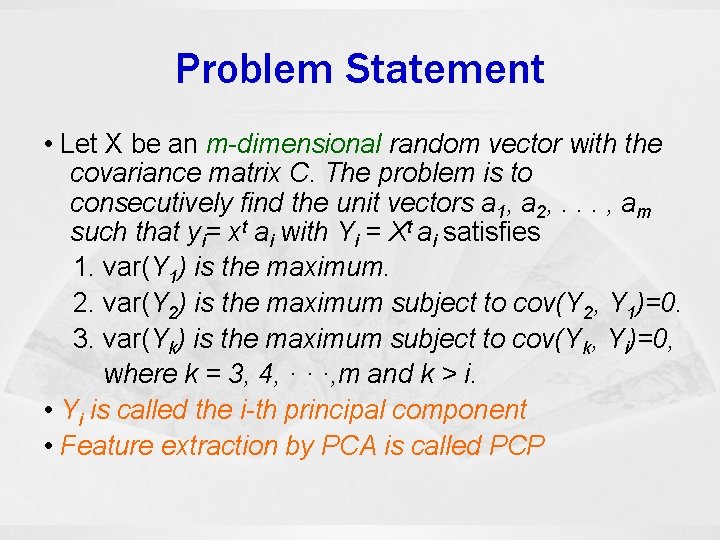
Problem Statement • Let X be an m-dimensional random vector with the covariance matrix C. The problem is to consecutively find the unit vectors a 1, a 2, . . . , am such that yi= xt ai with Yi = Xt ai satisfies 1. var(Y 1) is the maximum. 2. var(Y 2) is the maximum subject to cov(Y 2, Y 1)=0. 3. var(Yk) is the maximum subject to cov(Yk, Yi)=0, where k = 3, 4, · · ·, m and k > i. • Yi is called the i-th principal component • Feature extraction by PCA is called PCP

The Solutions ß ß ß Let (λi, ui) be the pairs of eigenvalues and eigenvectors of the covariance matrix C such that λ 1 ≥ λ 2 ≥. . . ≥ λm ( ≥ 0 ) and ∥u i ∥ 2 = 1, ∀ 1 ≤ i ≤. m Then ai = ui and var(Yi)=λi for 1 ≤ i ≤ m.

Computations Given n observations x 1, x 2, . . . , xn of mdimensional column vectors 1. Compute the mean vector μ = (x 1+x 2+. . . +xn )/n 2. Compute the covariance matrix by MLE C = (1/n) Σi=1 n (xi − μ)t 3. Compute the eigenvalue/eigenvector pairs (λi, ui) of C with λ 1 ≥ λ 2 ≥. . . ≥ λm ( ≥ 0 ) 4. Compute the first d principal components yi(j) = xit uj, for each observation xi, 1 ≤ i ≤ n, along the direction uj , j = 1, 2, · · · , d. 5. (λ 1 +λ 2 +. . . + λd)/ (λ 1 +λ 2 +. . . + λd +. . . + λm) > 85%

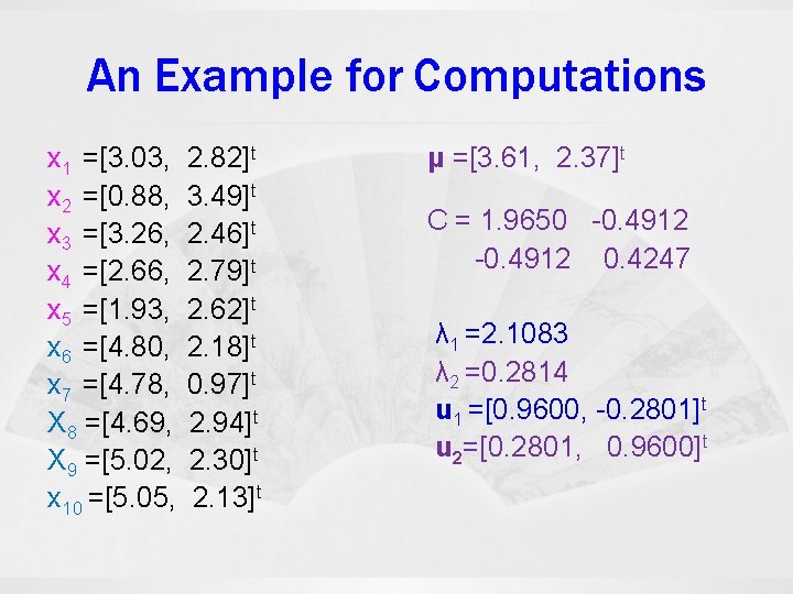
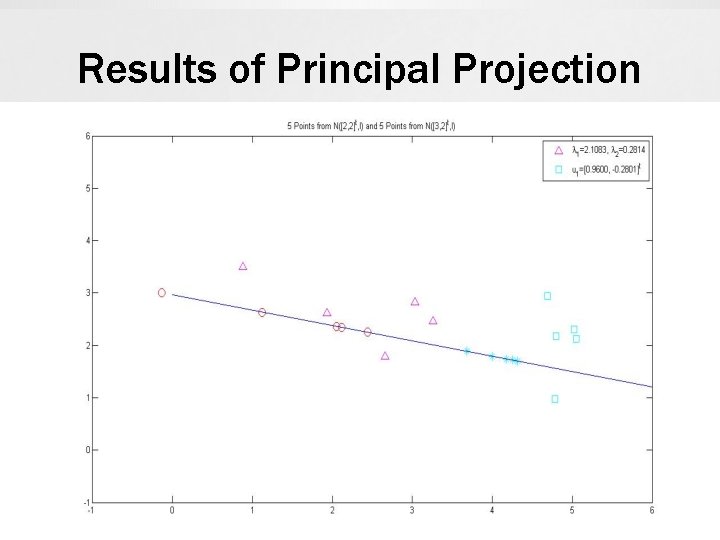
An Example for Computations x 1 =[3. 03, x 2 =[0. 88, x 3 =[3. 26, x 4 =[2. 66, x 5 =[1. 93, x 6 =[4. 80, x 7 =[4. 78, X 8 =[4. 69, X 9 =[5. 02, x 10 =[5. 05, 2. 82]t 3. 49]t 2. 46]t 2. 79]t 2. 62]t 2. 18]t 0. 97]t 2. 94]t 2. 30]t 2. 13]t μ =[3. 61, 2. 37]t C = 1. 9650 -0. 4912 0. 4247 λ 1 =2. 1083 λ 2 =0. 2814 u 1 =[0. 9600, -0. 2801]t u 2=[0. 2801, 0. 9600]t

Results of Principal Projection

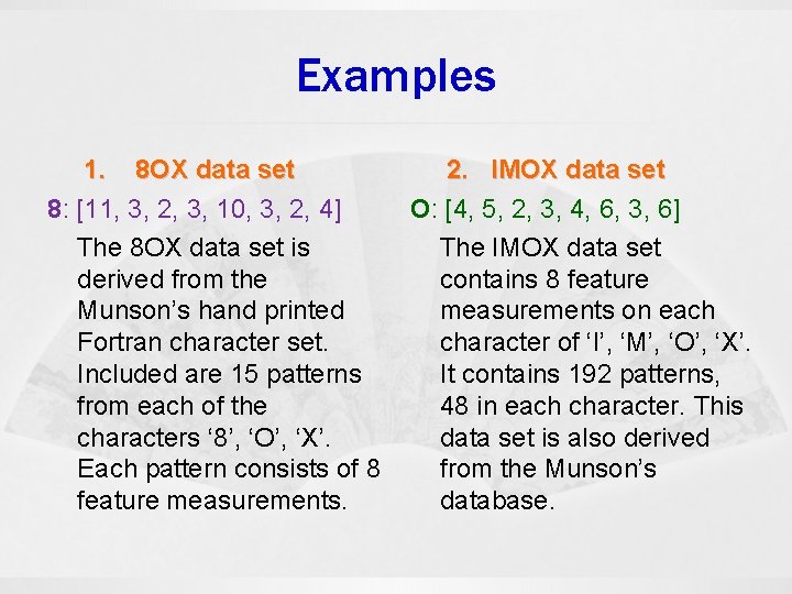
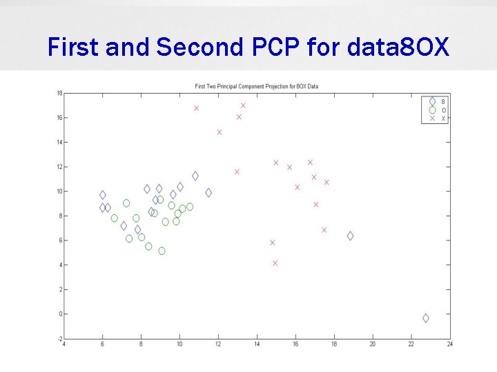
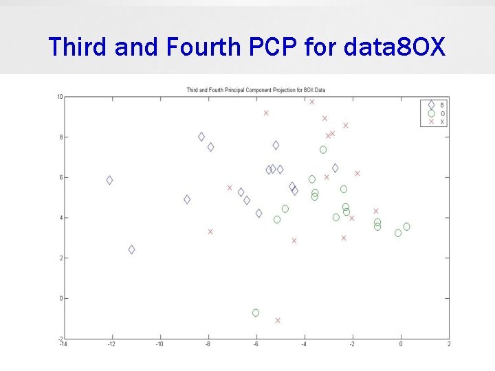
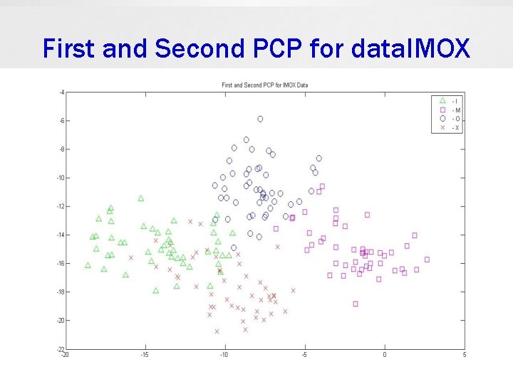
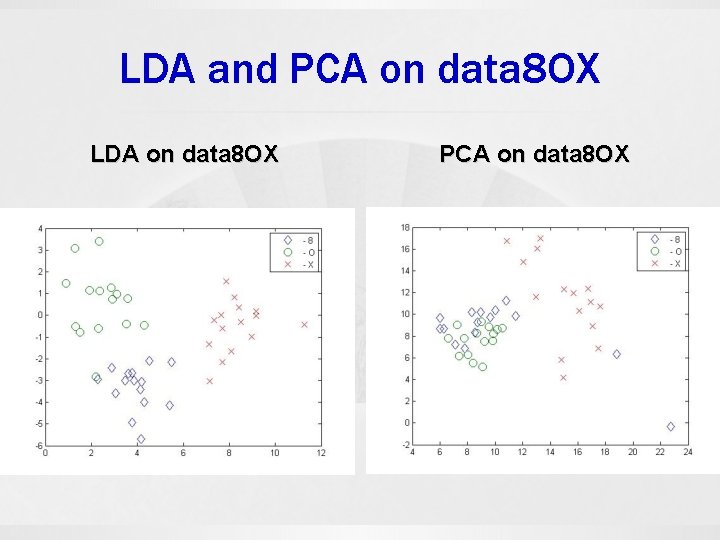
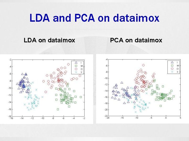
Examples 1. 8 OX data set 8: [11, 3, 2, 3, 10, 3, 2, 4] The 8 OX data set is derived from the Munson’s hand printed Fortran character set. Included are 15 patterns from each of the characters ‘ 8’, ‘O’, ‘X’. Each pattern consists of 8 feature measurements. 2. IMOX data set O: [4, 5, 2, 3, 4, 6, 3, 6] The IMOX data set contains 8 feature measurements on each character of ‘I’, ‘M’, ‘O’, ‘X’. It contains 192 patterns, 48 in each character. This data set is also derived from the Munson’s database.

First and Second PCP for data 8 OX

Third and Fourth PCP for data 8 OX

First and Second PCP for data. IMOX

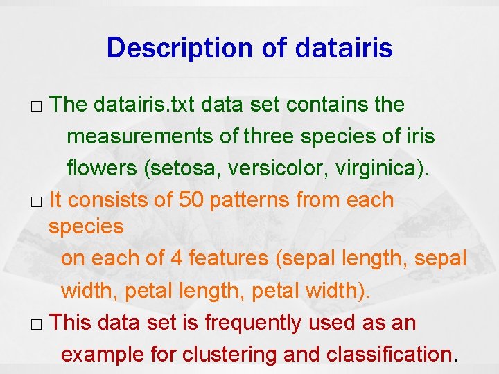
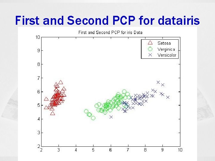
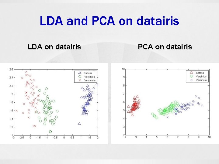
Description of datairis □ The datairis. txt data set contains the measurements of three species of iris flowers (setosa, versicolor, virginica). □ It consists of 50 patterns from each species on each of 4 features (sepal length, sepal width, petal length, petal width). □ This data set is frequently used as an example for clustering and classification.

First and Second PCP for datairis

Example that PCP is Not Working PCP works as expected PCP is not working as expected

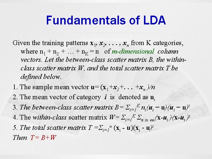
Fundamentals of LDA Given the training patterns x 1, x 2, . . . , xn from K categories, where n 1 + n 2 + … + n. K = n of m-dimensional column vectors. Let the between-class scatter matrix B, the withinclass scatter matrix W, and the total scatter matrix T be defined below. 1. The sample mean vector u= (x 1+x 2+. . . +xn )/n 2. The mean vector of category i is denoted as ui 3. The between-class scatter matrix B= Σi=1 K ni(ui − u)t 4. The within-class scatter matrix W= Σi=1 K Σx in ωi(x-ui )t 5. The total scatter matrix T =Σi=1 n (xi - u)t Then T= B+W

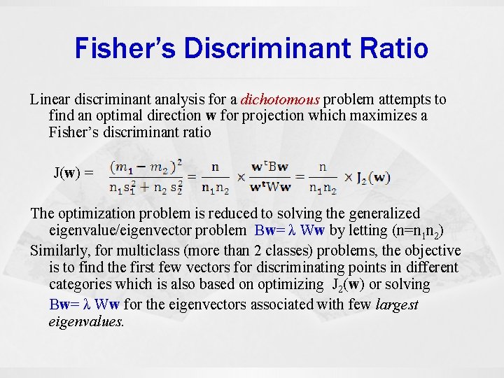
Fisher’s Discriminant Ratio Linear discriminant analysis for a dichotomous problem attempts to find an optimal direction w for projection which maximizes a Fisher’s discriminant ratio J(w) = The optimization problem is reduced to solving the generalized eigenvalue/eigenvector problem Bw= λ Ww by letting (n=n 1 n 2) Similarly, for multiclass (more than 2 classes) problems, the objective is to find the first few vectors for discriminating points in different categories which is also based on optimizing J 2(w) or solving Bw= λ Ww for the eigenvectors associated with few largest eigenvalues.

Fundamentals of LDA

LDA and PCA on data 8 OX LDA on data 8 OX PCA on data 8 OX

LDA and PCA on dataimox LDA on dataimox PCA on dataimox

LDA and PCA on datairis LDA on datairis PCA on datairis

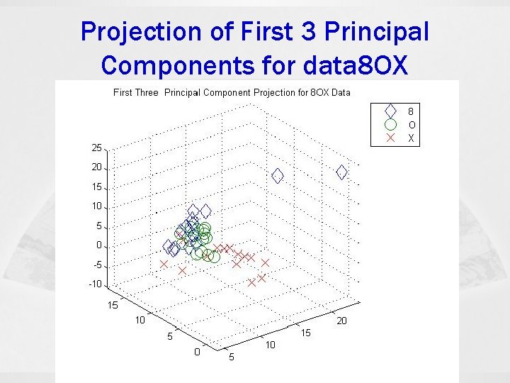
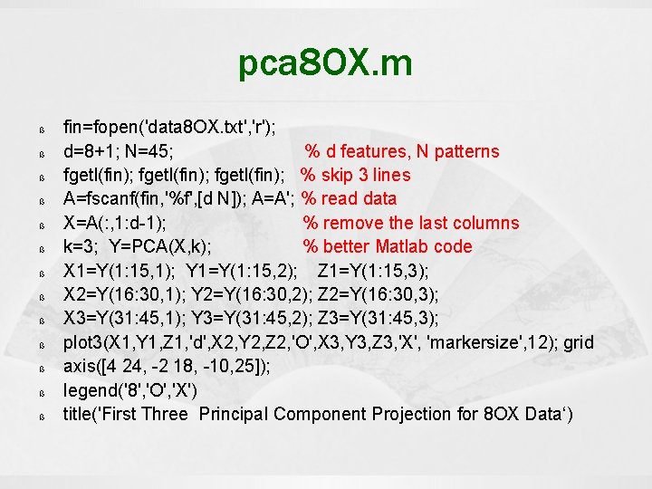
Projection of First 3 Principal Components for data 8 OX

pca 8 OX. m ß ß ß ß fin=fopen('data 8 OX. txt', 'r'); d=8+1; N=45; % d features, N patterns fgetl(fin); % skip 3 lines A=fscanf(fin, '%f', [d N]); A=A'; % read data X=A(: , 1: d-1); % remove the last columns k=3; Y=PCA(X, k); % better Matlab code X 1=Y(1: 15, 1); Y 1=Y(1: 15, 2); Z 1=Y(1: 15, 3); X 2=Y(16: 30, 1); Y 2=Y(16: 30, 2); Z 2=Y(16: 30, 3); X 3=Y(31: 45, 1); Y 3=Y(31: 45, 2); Z 3=Y(31: 45, 3); plot 3(X 1, Y 1, Z 1, 'd', X 2, Y 2, Z 2, 'O', X 3, Y 3, Z 3, 'X', 'markersize', 12); grid axis([4 24, -2 18, -10, 25]); legend('8', 'O', 'X') title('First Three Principal Component Projection for 8 OX Data‘)

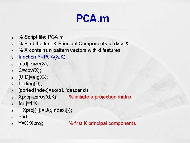
PCA. m ß ß ß ß % Script file: PCA. m % Find the first K Principal Components of data X % X contains n pattern vectors with d features function Y=PCA(X, K) [n, d]=size(X); C=cov(X); [U D]=eig(C); L=diag(D); [sorted index]=sort(L, 'descend'); Xproj=zeros(d, K); % initiate a projection matrix for j=1: K Xproj(: , j)=U(: , index(j)); end Y=X*Xproj; % first K principal components