Canonical Discriminant Analysis for Classification and Prediction Discriminant

Canonical Discriminant Analysis for Classification and Prediction

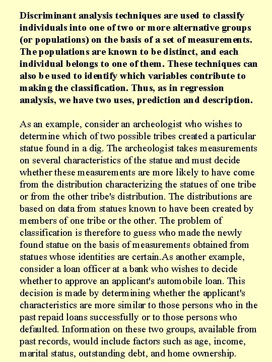
Discriminant analysis techniques are used to classify individuals into one of two or more alternative groups (or populations) on the basis of a set of measurements. The populations are known to be distinct, and each individual belongs to one of them. These techniques can also be used to identify which variables contribute to making the classification. Thus, as in regression analysis, we have two uses, prediction and description. As an example, consider an archeologist who wishes to determine which of two possible tribes created a particular statue found in a dig. The archeologist takes measurements on several characteristics of the statue and must decide whether these measurements are more likely to have come from the distribution characterizing the statues of one tribe or from the other tribe's distribution. The distributions are based on data from statues known to have been created by members of one tribe or the other. The problem of classification is therefore to guess who made the newly found statue on the basis of measurements obtained from statues whose identities are certain. As another example, consider a loan officer at a bank who wishes to decide whether to approve an applicant's automobile loan. This decision is made by determining whether the applicant's characteristics are more similar to those persons who in the past repaid loans successfully or to those persons who defaulted. Information on these two groups, available from past records, would include factors such as age, income, marital status, outstanding debt, and home ownership.

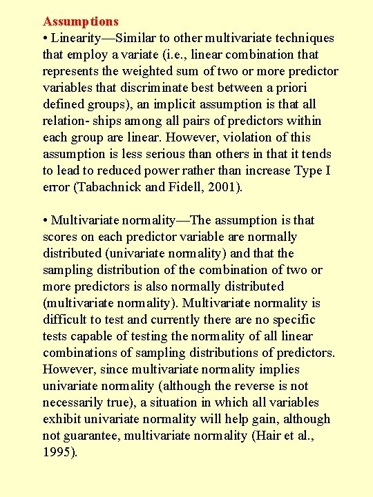
Assumptions • Linearity—Similar to other multivariate techniques that employ a variate (i. e. , linear combination that represents the weighted sum of two or more predictor variables that discriminate best between a priori defined groups), an implicit assumption is that all relation- ships among all pairs of predictors within each group are linear. However, violation of this assumption is less serious than others in that it tends to lead to reduced power rather than increase Type I error (Tabachnick and Fidell, 2001). • Multivariate normality—The assumption is that scores on each predictor variable are normally distributed (univariate normality) and that the sampling distribution of the combination of two or more predictors is also normally distributed (multivariate normality). Multivariate normality is difficult to test and currently there are no specific tests capable of testing the normality of all linear combinations of sampling distributions of predictors. However, since multivariate normality implies univariate normality (although the reverse is not necessarily true), a situation in which all variables exhibit univariate normality will help gain, although not guarantee, multivariate normality (Hair et al. , 1995).

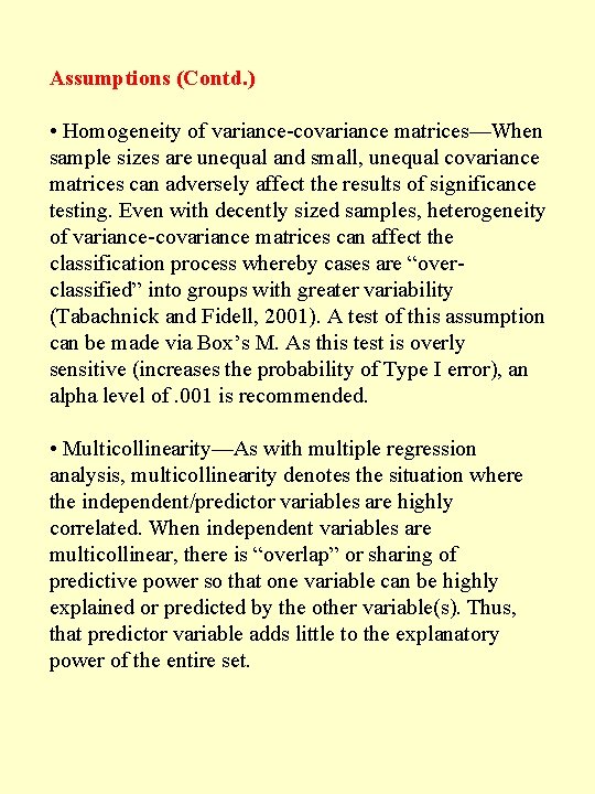
Assumptions (Contd. ) • Homogeneity of variance-covariance matrices—When sample sizes are unequal and small, unequal covariance matrices can adversely affect the results of significance testing. Even with decently sized samples, heterogeneity of variance-covariance matrices can affect the classification process whereby cases are “overclassified” into groups with greater variability (Tabachnick and Fidell, 2001). A test of this assumption can be made via Box’s M. As this test is overly sensitive (increases the probability of Type I error), an alpha level of. 001 is recommended. • Multicollinearity—As with multiple regression analysis, multicollinearity denotes the situation where the independent/predictor variables are highly correlated. When independent variables are multicollinear, there is “overlap” or sharing of predictive power so that one variable can be highly explained or predicted by the other variable(s). Thus, that predictor variable adds little to the explanatory power of the entire set.

Application Areas 1. The major application area for this technique is where we want to be able to distinguish between two or more sets of objects or people, based on the knowledge of some of their characteristics. 2. Examples include the selection process for a job, the admission process of an educational programme in a college, or dividing a group of people into potential buyers and non-buyers. 3. Discriminant analysis can be, and is in fact used, by credit rating agencies to rate individuals, to classify them into good lending risks or bad lending risks. The detailed example discussed later tells you how to do that. 4. To summarize, we can use discriminant analysis when we have a nominal dependent variable, such as to classify objects into two or more groups based on the knowledge of some variables (characteristics) related to them. Typically, these groups would be users-nonusers, potentially successful salesman – potentially unsuccessful salesman, high risk – low risk consumer, or on similar lines.

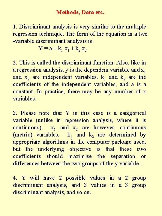
Methods, Data etc. 1. Discriminant analysis is very similar to the multiple regression technique. The form of the equation in a two -variable discriminant analysis is: Y = a + k 1 x 1 + k 2 x 2 2. This is called the discriminant function. Also, like in a regression analysis, y is the dependent variable and x 1 and x 2 are independent variables. k 1 and k 2 are the coefficients of the independent variables, and a is a constant. In practice, there may be any number of x variables. 3. Please note that Y in this case is a categorical variable (unlike in regression analysis, where it is continuous). x 1 and x 2 are however, continuous (metric) variables. k 1 and k 2 are determined by appropriate algorithms in the computer package used, but the underlying objective is that these two coefficients should maximise the separation or differences between the two groups of the y variable. 4. Y will have 2 possible values in a 2 group discriminant analysis, and 3 values in a 3 group discriminant analysis, and so on.

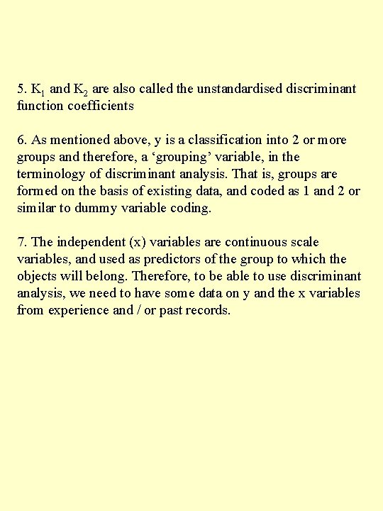
5. K 1 and K 2 are also called the unstandardised discriminant function coefficients 6. As mentioned above, y is a classification into 2 or more groups and therefore, a ‘grouping’ variable, in the terminology of discriminant analysis. That is, groups are formed on the basis of existing data, and coded as 1 and 2 or similar to dummy variable coding. 7. The independent (x) variables are continuous scale variables, and used as predictors of the group to which the objects will belong. Therefore, to be able to use discriminant analysis, we need to have some data on y and the x variables from experience and / or past records.

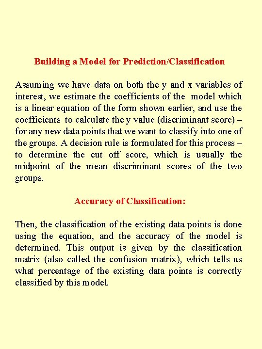
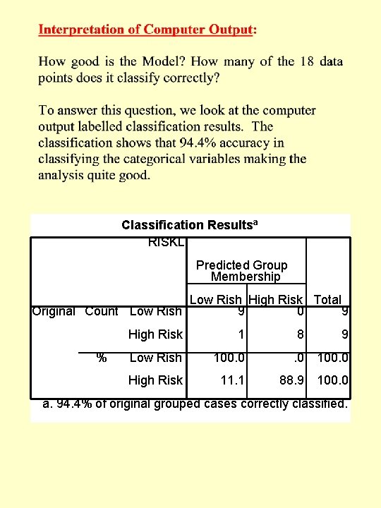
Building a Model for Prediction/Classification Assuming we have data on both the y and x variables of interest, we estimate the coefficients of the model which is a linear equation of the form shown earlier, and use the coefficients to calculate the y value (discriminant score) – for any new data points that we want to classify into one of the groups. A decision rule is formulated for this process – to determine the cut off score, which is usually the midpoint of the mean discriminant scores of the two groups. Accuracy of Classification: Then, the classification of the existing data points is done using the equation, and the accuracy of the model is determined. This output is given by the classification matrix (also called the confusion matrix), which tells us what percentage of the existing data points is correctly classified by this model.

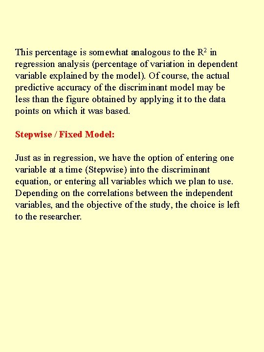
This percentage is somewhat analogous to the R 2 in regression analysis (percentage of variation in dependent variable explained by the model). Of course, the actual predictive accuracy of the discriminant model may be less than the figure obtained by applying it to the data points on which it was based. Stepwise / Fixed Model: Just as in regression, we have the option of entering one variable at a time (Stepwise) into the discriminant equation, or entering all variables which we plan to use. Depending on the correlations between the independent variables, and the objective of the study, the choice is left to the researcher.

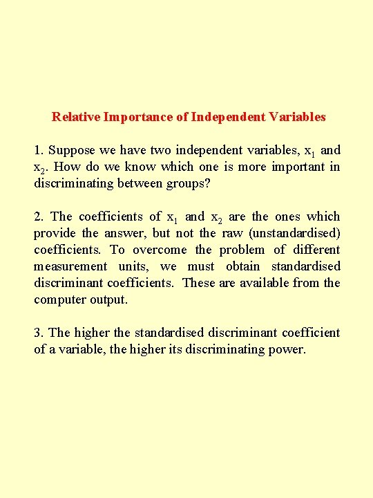
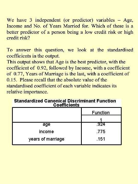
Relative Importance of Independent Variables 1. Suppose we have two independent variables, x 1 and x 2. How do we know which one is more important in discriminating between groups? 2. The coefficients of x 1 and x 2 are the ones which provide the answer, but not the raw (unstandardised) coefficients. To overcome the problem of different measurement units, we must obtain standardised discriminant coefficients. These are available from the computer output. 3. The higher the standardised discriminant coefficient of a variable, the higher its discriminating power.

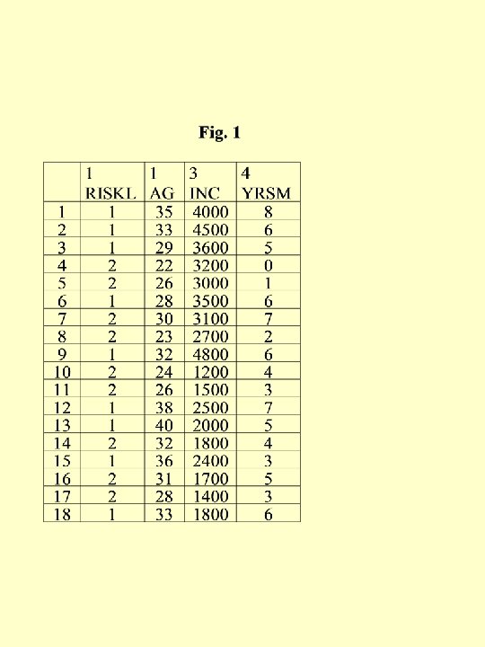
Example Suppose a Bank wants to start credit card division. They want to use discriminant analysis and set up a system to screen applicants and classify them as either ‘low risk’ or ‘high risk’ (risk of default on credit card bill payments), based on information collected from their applications for a credit card. Suppose the Bank has managed to get from another Bank, its sister bank, some data on their credit card holders who turned out to be ‘low risk’ (no default) and ‘high risk’ (defaulting on payments) customers. These data on 18 customers are given in fig. 1 (File: Discriminant. sav).

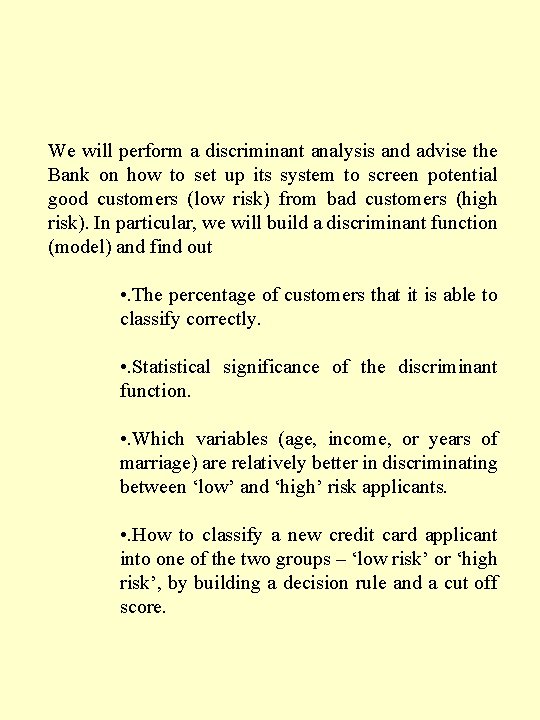
We will perform a discriminant analysis and advise the Bank on how to set up its system to screen potential good customers (low risk) from bad customers (high risk). In particular, we will build a discriminant function (model) and find out • . The percentage of customers that it is able to classify correctly. • . Statistical significance of the discriminant function. • . Which variables (age, income, or years of marriage) are relatively better in discriminating between ‘low’ and ‘high’ risk applicants. • . How to classify a new credit card applicant into one of the two groups – ‘low risk’ or ‘high risk’, by building a decision rule and a cut off score.

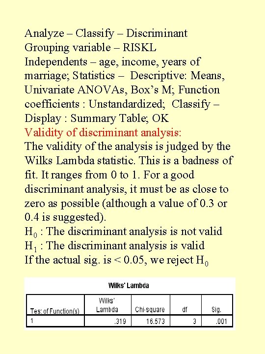
Analyze – Classify – Discriminant Grouping variable – RISKL Independents – age, income, years of marriage; Statistics – Descriptive: Means, Univariate ANOVAs, Box’s M; Function coefficients : Unstandardized; Classify – Display : Summary Table; OK Validity of discriminant analysis: The validity of the analysis is judged by the Wilks Lambda statistic. This is a badness of fit. It ranges from 0 to 1. For a good discriminant analysis, it must be as close to zero as possible (although a value of 0. 3 or 0. 4 is suggested). H 0 : The discriminant analysis is not valid H 1 : The discriminant analysis is valid If the actual sig. is < 0. 05, we reject H 0

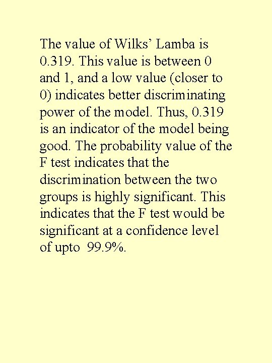
The value of Wilks’ Lamba is 0. 319. This value is between 0 and 1, and a low value (closer to 0) indicates better discriminating power of the model. Thus, 0. 319 is an indicator of the model being good. The probability value of the F test indicates that the discrimination between the two groups is highly significant. This indicates that the F test would be significant at a confidence level of upto 99. 9%.

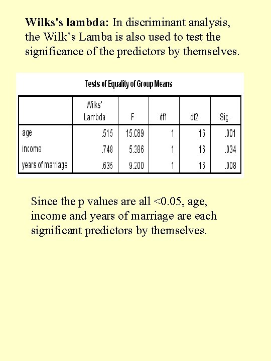
Wilks's lambda: In discriminant analysis, the Wilk’s Lamba is also used to test the significance of the predictors by themselves. Since the p values are all <0. 05, age, income and years of marriage are each significant predictors by themselves.

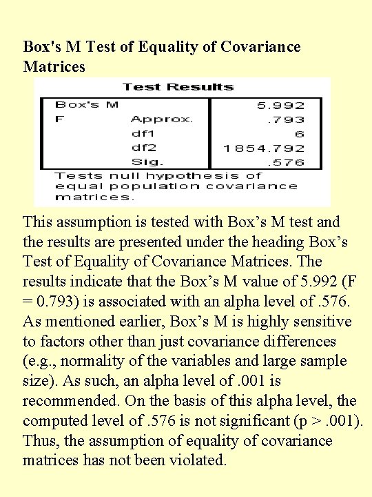
Box's M Test of Equality of Covariance Matrices This assumption is tested with Box’s M test and the results are presented under the heading Box’s Test of Equality of Covariance Matrices. The results indicate that the Box’s M value of 5. 992 (F = 0. 793) is associated with an alpha level of. 576. As mentioned earlier, Box’s M is highly sensitive to factors other than just covariance differences (e. g. , normality of the variables and large sample size). As such, an alpha level of. 001 is recommended. On the basis of this alpha level, the computed level of. 576 is not significant (p >. 001). Thus, the assumption of equality of covariance matrices has not been violated.

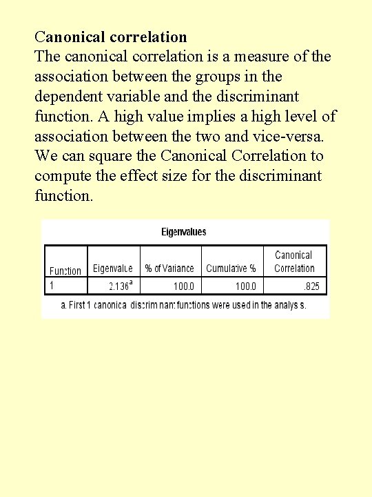
Canonical correlation The canonical correlation is a measure of the association between the groups in the dependent variable and the discriminant function. A high value implies a high level of association between the two and vice-versa. We can square the Canonical Correlation to compute the effect size for the discriminant function.

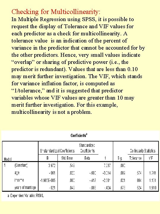
Checking for Multicollinearity: In Multiple Regression using SPSS, it is possible to request the display of Tolerance and VIF values for each predictor as a check for multicollinearity. A tolerance value is an indication of the percent of variance in the predictor that cannot be accounted for by the other predictors. Hence, very small values indicate “overlap” or sharing of predictive power (i. e. , the predictor is redundant). Values that are less than 0. 10 may merit further investigation. The VIF, which stands for variance inflation factor, is computed as “ 1/tolerance, ” and it is suggested that predictor variables whose VIF values are greater than 10 may merit further investigation. For this example, multicollinearity is not a problem.

Classification Resultsa RISKL Predicted Group Membership Low Rish High Risk Total Original Count Low Rish 9 0 9 % High Risk 1 8 9 Low Rish 100. 0 High Risk 11. 1 88. 9 100. 0 a. 94. 4% of original grouped cases correctly classified.

Standardized Canonical Discriminant Function Coefficients Function age 1. 924 income . 775 years of marriage . 151

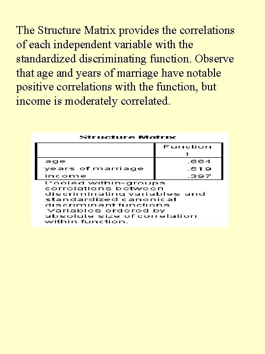
The Structure Matrix provides the correlations of each independent variable with the standardized discriminating function. Observe that age and years of marriage have notable positive correlations with the function, but income is moderately correlated.

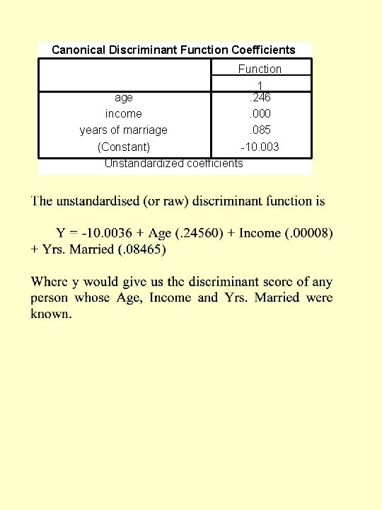
Canonical Discriminant Function Coefficients Function 1 age. 246 income. 000 years of marriage. 085 (Constant) -10. 003 Unstandardized coefficients

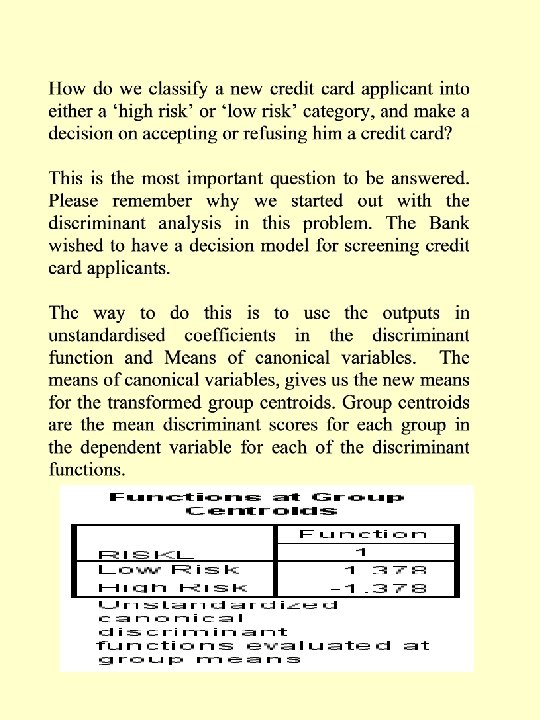
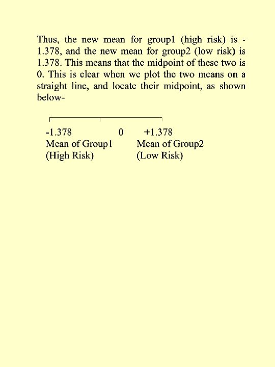
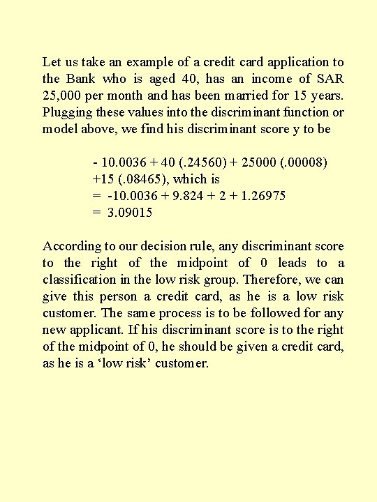
Let us take an example of a credit card application to the Bank who is aged 40, has an income of SAR 25, 000 per month and has been married for 15 years. Plugging these values into the discriminant function or model above, we find his discriminant score y to be - 10. 0036 + 40 (. 24560) + 25000 (. 00008) +15 (. 08465), which is = -10. 0036 + 9. 824 + 2 + 1. 26975 = 3. 09015 According to our decision rule, any discriminant score to the right of the midpoint of 0 leads to a classification in the low risk group. Therefore, we can give this person a credit card, as he is a low risk customer. The same process is to be followed for any new applicant. If his discriminant score is to the right of the midpoint of 0, he should be given a credit card, as he is a ‘low risk’ customer.