Predictive vs Reactive Control Dr Nathan Dalrymple Space

Predictive vs. Reactive Control Dr. Nathan Dalrymple Space Vehicles Directorate Air Force Research Laboratory Timothy Henry National Solar Observatory 10 Dec 2004 ATST M 1 Workshop

Goals of Prediction • Overall: Predict temperature far enough in advance that M 1 can react and keep surface temperature in “green zone” • Recall: Whiz-bang controller will put the mirror in the green zone with accurate Te prediction • Specific: How? Using what algorithm? • Specific: How well can we do using our best algorithm? • Is the predictive control approach a viable solution?

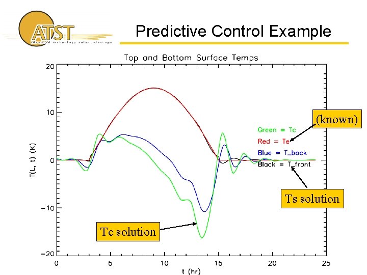
Predictive Control Example (known) Ts solution Tc solution

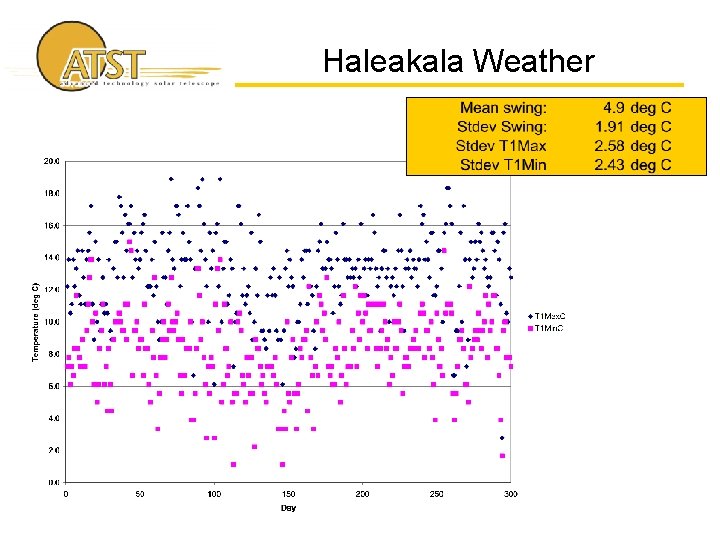
Haleakala Weather

Methods Tried • • • Persistence forecast Moving linear fit Moving quadratic fit Database shape fit Nearest Neighbor

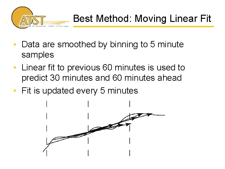
Best Method: Moving Linear Fit • Data are smoothed by binning to 5 minute samples • Linear fit to previous 60 minutes is used to predict 30 minutes and 60 minutes ahead • Fit is updated every 5 minutes

Linear Prediction Results Mean % in “green zone”: 50. 3 Stdev % in “green zone”: 7. 9 Not good enough. Note: the Subaru group on Mauna Kea tried a similar exercise using nighttime data, and arrived at nearly identical results. See Miyashita et al. , Proc. SPIE Vol. 4837, p. 255, 2003.

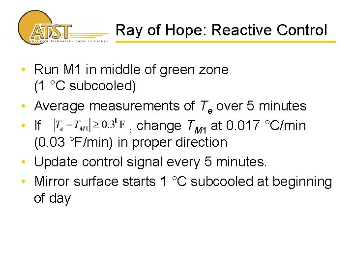
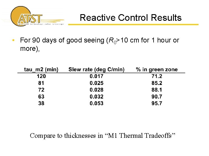
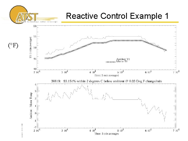
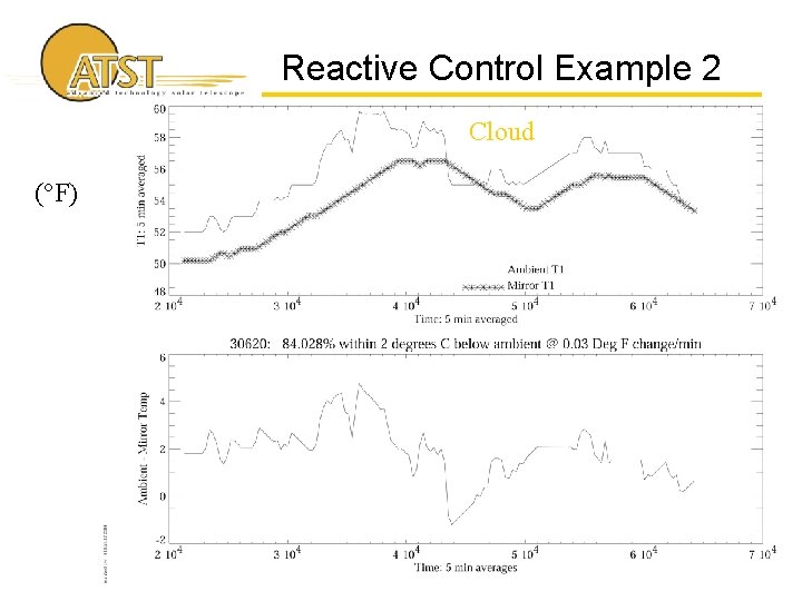
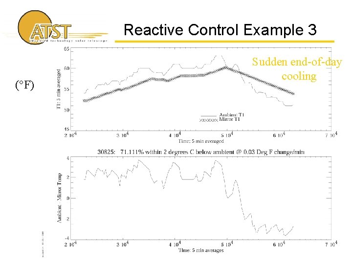
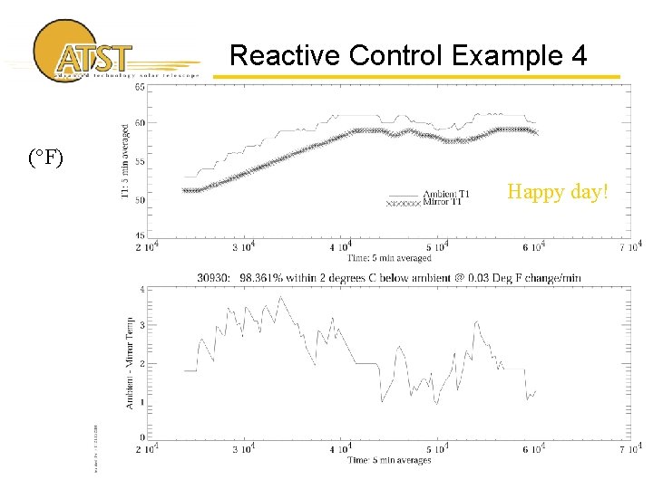
Ray of Hope: Reactive Control • Run M 1 in middle of green zone (1 °C subcooled) • Average measurements of Te over 5 minutes • If , change TM 1 at 0. 017 °C/min (0. 03 °F/min) in proper direction • Update control signal every 5 minutes. • Mirror surface starts 1 °C subcooled at beginning of day

Reactive Control Results • For 90 days of good seeing (R 0>10 cm for 1 hour or more), Compare to thicknesses in “M 1 Thermal Tradeoffs”

Reactive Control Example 1 (°F)

Reactive Control Example 2 Cloud (°F)

Reactive Control Example 3 (°F) Sudden end-of-day cooling

Reactive Control Example 4 (°F) Happy day!

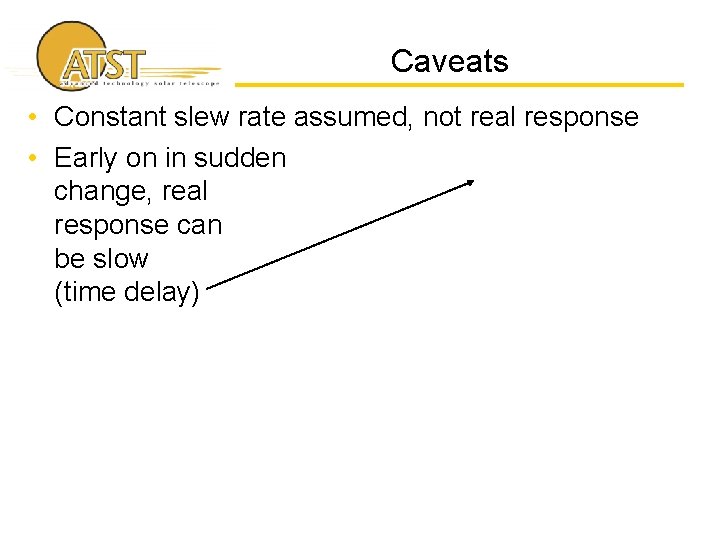
Caveats • Constant slew rate assumed, not real response • Early on in sudden change, real response can be slow (time delay)

Summary • At this point, reactive closed-loop control looks like the winner—a 75 mm, air-cooled mirror responds rapidly enough to be in the green zone 96 % of the time on good seeing days. • We cannot predict Te to better than about 50% of the time.

Next Steps • Build a MATLAB/Simulink or similar control system model, including real mirror response and typical Te(t) curves • Use Simulink model to refine estimate of mirror thickness and thermal control system