M 1 Thermal Control Dr Nathan Dalrymple Space

M 1 Thermal Control Dr. Nathan Dalrymple Space Vehicles Directorate Air Force Research Laboratory 28 Oct 2005 ATST M 1 Workshop

Outline • • Motivation and Requirements Problem Setup PID control Results

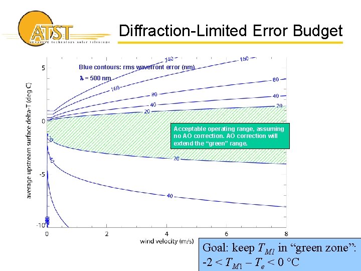
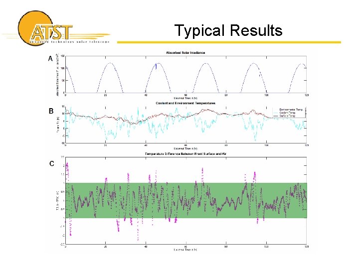
Diffraction-Limited Error Budget Blue contours: rms wavefront error (nm) l = 500 nm Acceptable operating range, assuming no AO correction will extend the “green” range. Goal: keep TM 1 in “green zone”: -2 < TM 1 – Te < 0 °C

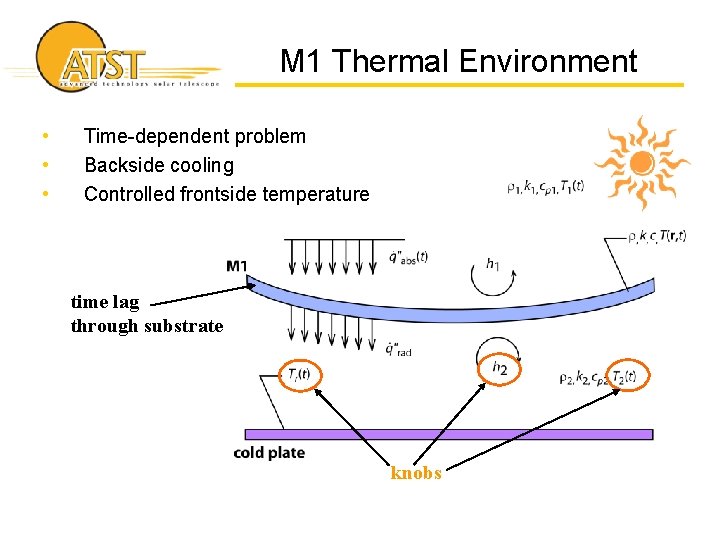
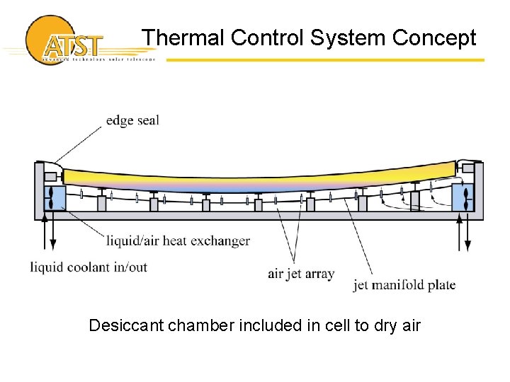
M 1 Thermal Environment • • • Time-dependent problem Backside cooling Controlled frontside temperature time lag through substrate knobs

Thermal Control System Concept Desiccant chamber included in cell to dry air

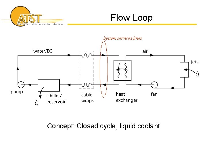
Flow Loop System services lines Concept: Closed cycle, liquid coolant

M 1 Thermal Modeling • Modeling hierarchy – – 0 D, t “Lumped capacity” 1 D, t the workhorse 2 D, t support pad effects 3 D, t mirror edge effects • Control system models

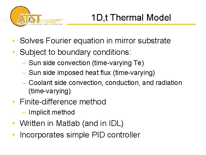
1 D, t Thermal Model • Solves Fourier equation in mirror substrate • Subject to boundary conditions: – Sun side convection (time-varying Te) – Sun side imposed heat flux (time-varying) – Coolant side convection, conduction, and radiation (time-varying) • Finite-difference method – Implicit method • Written in Matlab (and in IDL) • Incorporates simple PID controller

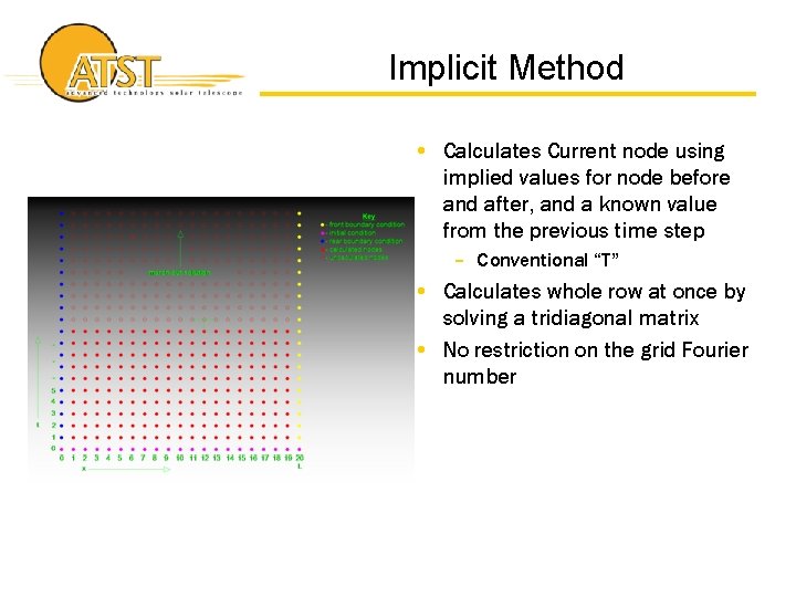
Implicit Method • Calculates Current node using implied values for node before and after, and a known value from the previous time step – Conventional “T” • Calculates whole row at once by solving a tridiagonal matrix • No restriction on the grid Fourier number

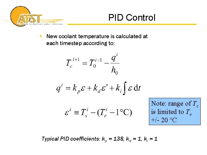
PID Control • New coolant temperature is calculated at each timestep according to: Note: range of Tc is limited to Te +/- 20 °C Typical PID coefficients: kp = 138, kd = 1, ki = 1

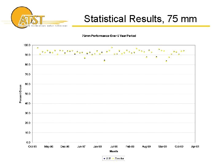
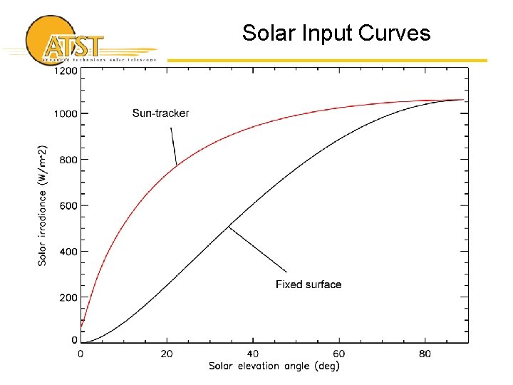
Input Data & Statistics • Ran model for 5 years from 1996 – 2000 • Used weather data from Hameteo station on Haleakala • Notes: – Used light curve from Hameteo sensor, which apparently is not a sun-tracker • Shape of solar heat flux curve is changed – Statistics may include nighttime (must check on this) – Statistics do include cloudy periods

Typical Results

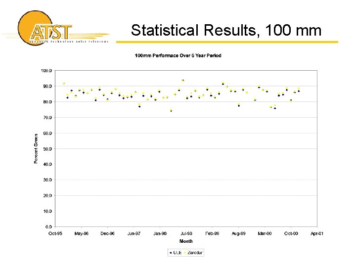
Statistical Results, 100 mm

Statistical Results, 75 mm

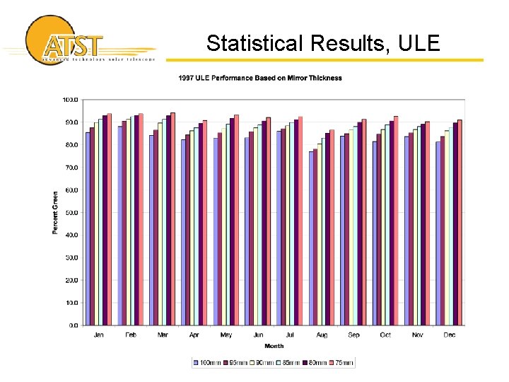
Statistical Results, ULE

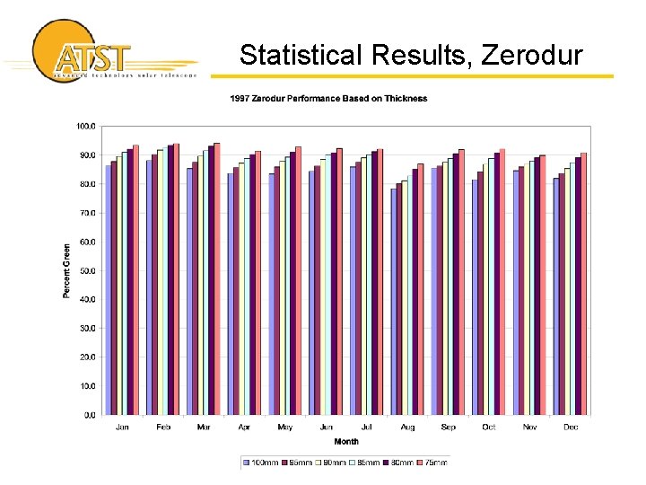
Statistical Results, Zerodur

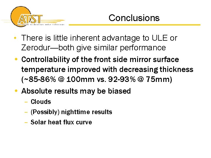
Conclusions • There is little inherent advantage to ULE or Zerodur—both give similar performance • Controllability of the front side mirror surface temperature improved with decreasing thickness (~85 -86% @ 100 mm vs. 92 -93% @ 75 mm) • Absolute results may be biased – Clouds – (Possibly) nighttime results – Solar heat flux curve

Backup Slides

Solar Input Curves

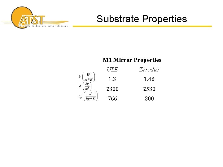
Substrate Properties M 1 Mirror Properties ULE Zerodur 1. 3 1. 46 2300 2530 766 800