Perfect Competition Copyright 2004 SouthWestern 14 Perfectly Competitive

Perfect Competition Copyright© 2004 South-Western 14

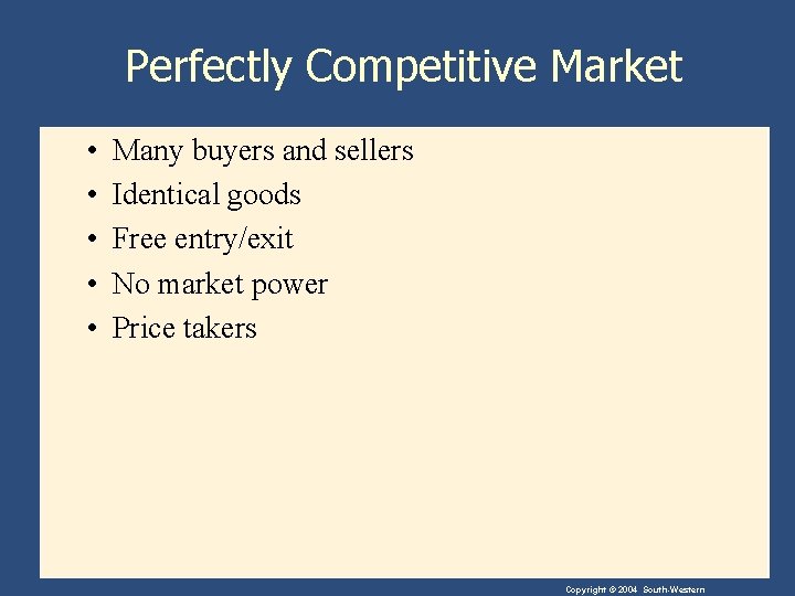
Perfectly Competitive Market • • • Many buyers and sellers Identical goods Free entry/exit No market power Price takers Copyright © 2004 South-Western

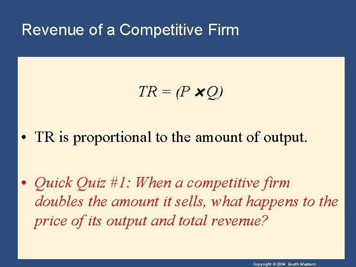
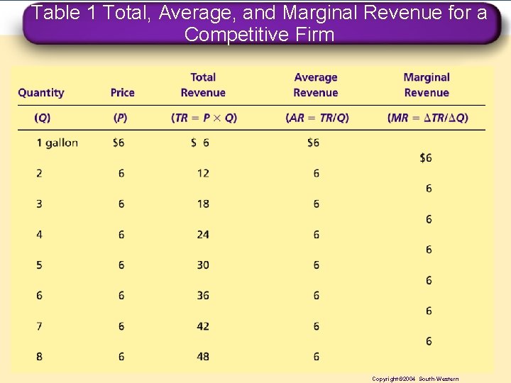
Revenue of a Competitive Firm TR = (P Q) • TR is proportional to the amount of output. • Quick Quiz #1: When a competitive firm doubles the amount it sells, what happens to the price of its output and total revenue? Copyright © 2004 South-Western

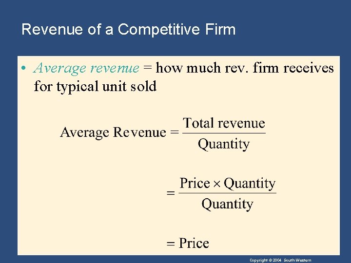
Revenue of a Competitive Firm • Average revenue = how much rev. firm receives for typical unit sold Copyright © 2004 South-Western

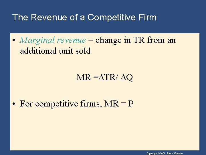
The Revenue of a Competitive Firm • Marginal revenue = change in TR from an additional unit sold MR = TR/ Q • For competitive firms, MR = P Copyright © 2004 South-Western

Table 1 Total, Average, and Marginal Revenue for a Competitive Firm Copyright© 2004 South-Western

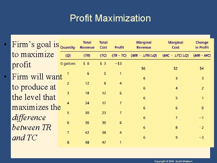
Profit Maximization • Firm’s goal is to maximize profit • Firm will want to produce at the level that maximizes the difference between TR and TC Copyright © 2004 South-Western

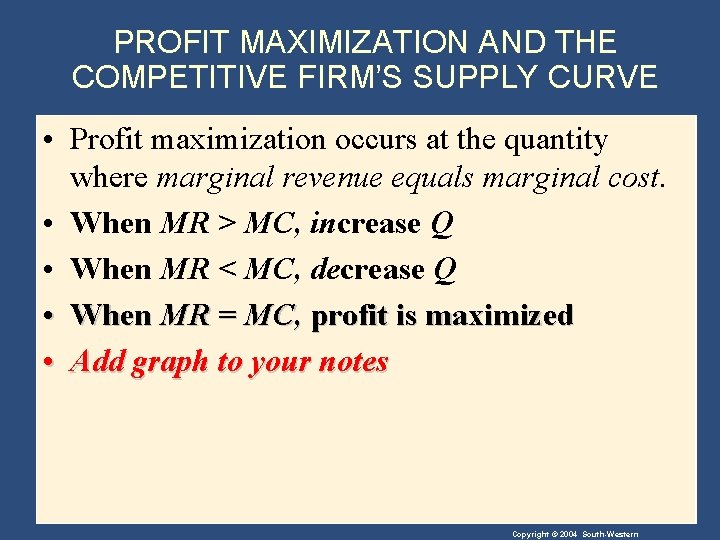
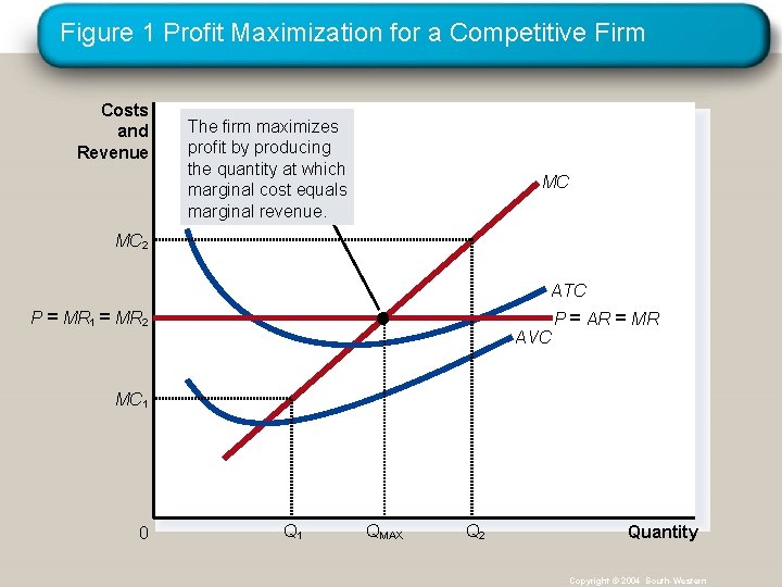
PROFIT MAXIMIZATION AND THE COMPETITIVE FIRM’S SUPPLY CURVE • Profit maximization occurs at the quantity where marginal revenue equals marginal cost. • When MR > MC, increase Q • When MR < MC, decrease Q • When MR = MC, profit is maximized • Add graph to your notes Copyright © 2004 South-Western

Figure 1 Profit Maximization for a Competitive Firm Costs and Revenue The firm maximizes profit by producing the quantity at which marginal cost equals marginal revenue. MC MC 2 ATC P = MR 1 = MR 2 AVC P = AR = MR MC 1 0 Q 1 QMAX Q 2 Quantity Copyright © 2004 South-Western

Firm’s Short-Run Decision to Shut Down or Exit • Shutdown = short-run decision not to produce anything during specific period of time b/c of current market conditions • Exit = long-run decision to leave market Copyright © 2004 South-Western

Firm’s Short-Run Decision to Shut Down • The firm considers its sunk costs when deciding to exit, but ignores them when deciding whether to shut down. • Sunk costs are costs that have already been committed and cannot be recovered. • The firm shuts down if the revenue it gets from producing is less than the variable cost of production. • Shut down if TR < VC • Shut down if TR/Q < VC/Q • Shut down if P < AVC Add graph to your notes Copyright © 2004 South-Western

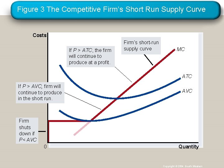
Figure 3 The Competitive Firm’s Short Run Supply Curve Costs If P > ATC, the firm will continue to produce at a profit. Firm’s short-run supply curve MC ATC If P > AVC, firm will continue to produce in the short run. AVC Firm shuts down if P< AVC 0 Quantity Copyright © 2004 South-Western

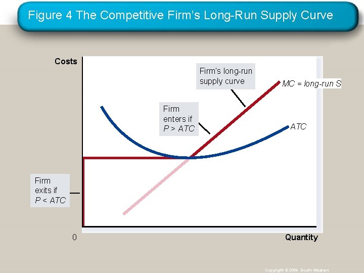
Firm’s Long-Run Decision to Exit • In the long run, the firm exits if the revenue it would get from producing is less than its total cost. • Exit if TR < TC • Exit if TR/Q < TC/Q • Exit if P < ATC Add graph to your notes • Entrepreneur will enter market if P > ATC Copyright © 2004 South-Western

Figure 4 The Competitive Firm’s Long-Run Supply Curve Costs Firm’s long-run supply curve Firm enters if P > ATC MC = long-run S ATC Firm exits if P < ATC 0 Quantity Copyright © 2004 South-Western

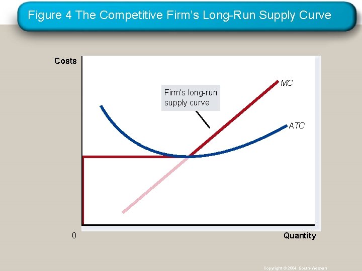
Figure 4 The Competitive Firm’s Long-Run Supply Curve Costs MC Firm’s long-run supply curve ATC 0 Quantity Copyright © 2004 South-Western

THE SUPPLY CURVE IN A COMPETITIVE MARKET • Short-Run Supply Curve • The portion of its marginal cost curve that lies above average variable cost. • Long-Run Supply Curve • The marginal cost curve above the minimum point of its average total cost curve. Copyright © 2004 South-Western

Quick Quiz #2 • How does a competitive firm determine its profit-maximizing level of output? Explain. • When does a profit-maximizing competitive firm decide to shut down? • When does it decide to exit a market? • Provide a graph that visually summarizes your responses. Copyright © 2004 South-Western

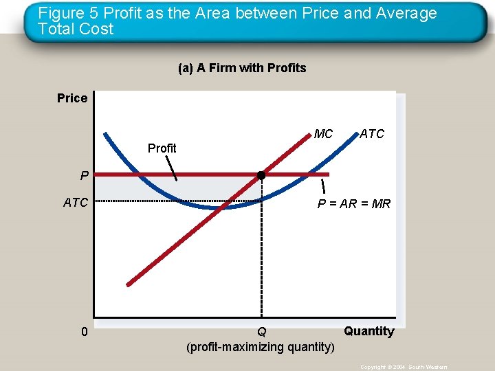
Figure 5 Profit as the Area between Price and Average Total Cost (a) A Firm with Profits Price MC ATC Profit P ATC P = AR = MR 0 Quantity Q (profit-maximizing quantity) Copyright © 2004 South-Western

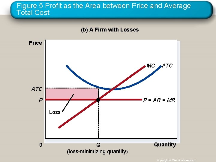
Figure 5 Profit as the Area between Price and Average Total Cost (b) A Firm with Losses Price MC ATC P P = AR = MR Loss 0 Q (loss-minimizing quantity) Quantity Copyright © 2004 South-Western

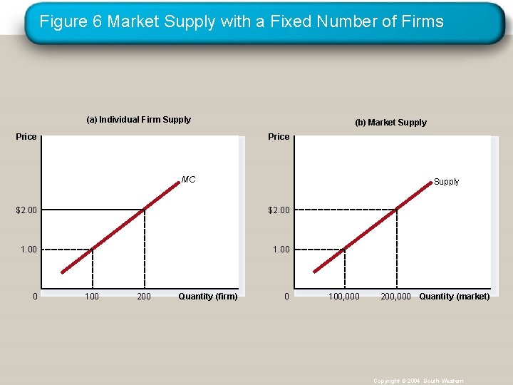
The Short Run: Market Supply with a Fixed Number of Firms • Market supply equals the sum of the quantities supplied by the individual firms in the market. • For any given price, each firm supplies a quantity of output so that its marginal cost equals price. • The market supply curve reflects the individual firms’ marginal cost curves. Add graphs to your notes Copyright © 2004 South-Western

Figure 6 Market Supply with a Fixed Number of Firms (a) Individual Firm Supply (b) Market Supply Price MC Supply $2. 00 1. 00 0 100 200 Quantity (firm) 0 100, 000 200, 000 Quantity (market) Copyright © 2004 South-Western

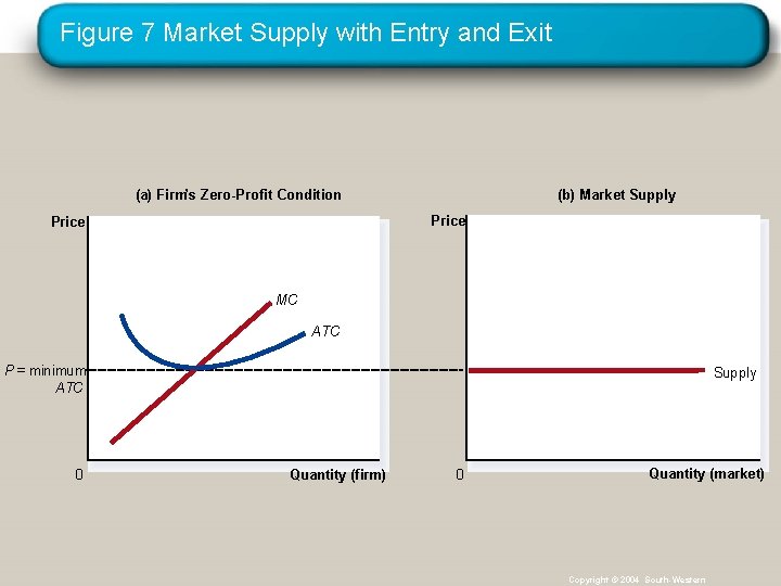
The Long Run: Market Supply with Entry and Exit • Firms will enter or exit the market until profit is driven to zero. • In the long-run, P = minimum ATC (efficient scale) • Long-run market supply curve is horizontal at this price. • After process of entry and exit ends, remaining firms must be making zero economic profit. • Recall that total cost includes opportunity costs. In zeroprofit equilibrium, firm’s revenue compensates owners for time and money they expend running business. Add graphs to your notes Copyright © 2004 South-Western

Figure 7 Market Supply with Entry and Exit (a) Firm’s Zero-Profit Condition (b) Market Supply Price MC ATC P = minimum ATC 0 Supply Quantity (firm) 0 Quantity (market) Copyright © 2004 South-Western

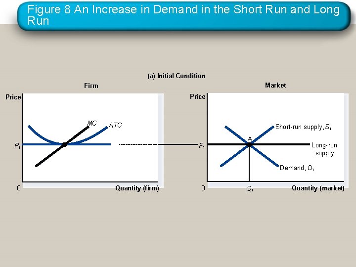
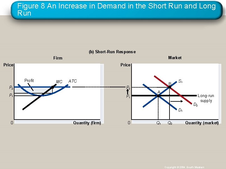
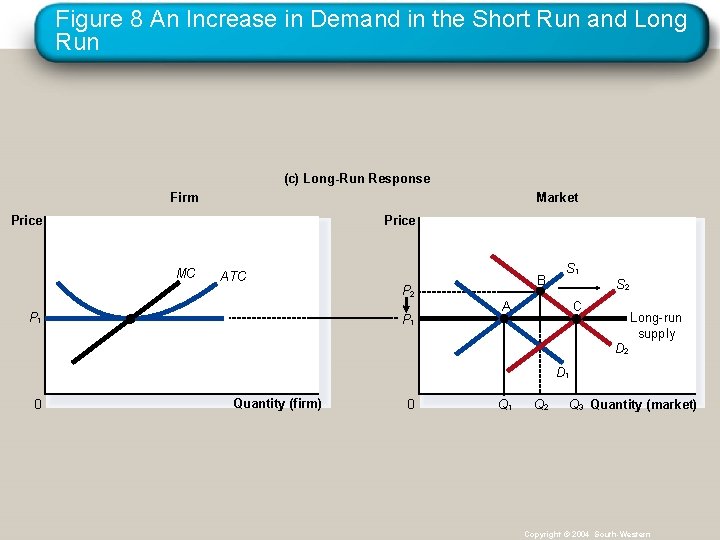
A Shift in Demand in the Short Run and Long Run • An increase in demand raises price and quantity in the short run. • Firms earn profits because price now exceeds average total cost. • Entry and exit occurs until firms are operating back at efficient scale. • Add graphs to your notes Copyright © 2004 South-Western

Figure 8 An Increase in Demand in the Short Run and Long Run (a) Initial Condition Market Firm Price MC ATC P 1 Short-run supply, S 1 P 1 A Long-run supply Demand, D 1 0 Quantity (firm) 0 Q 1 Quantity (market)

Figure 8 An Increase in Demand in the Short Run and Long Run (b) Short-Run Response Market Firm Price Profit MC ATC P 2 B P 2 P 1 S 1 A D 2 Long-run supply D 1 0 Quantity (firm) 0 Q 1 Q 2 Quantity (market) Copyright © 2004 South-Western

Figure 8 An Increase in Demand in the Short Run and Long Run (c) Long-Run Response Market Firm Price MC ATC P 1 B P 2 P 1 S 2 C A Long-run supply D 2 D 1 0 Quantity (firm) 0 Q 1 Q 2 Q 3 Quantity (market) Copyright © 2004 South-Western

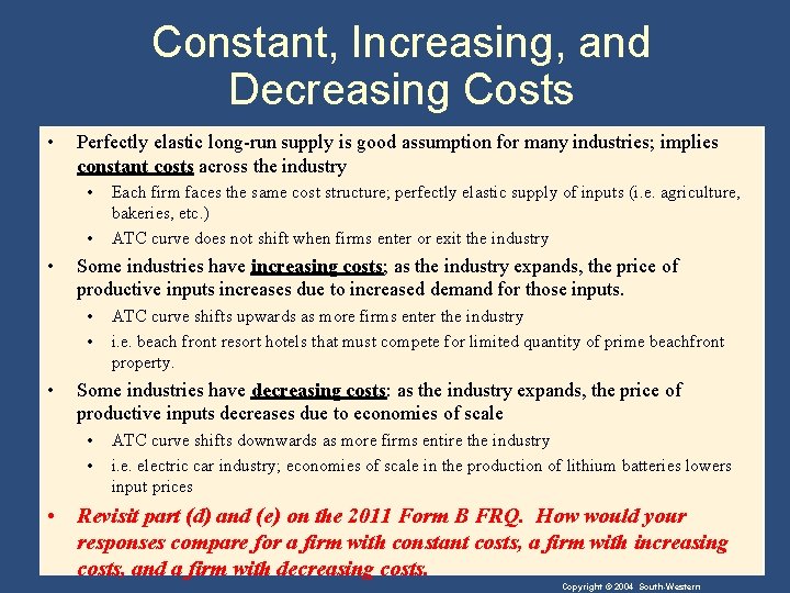
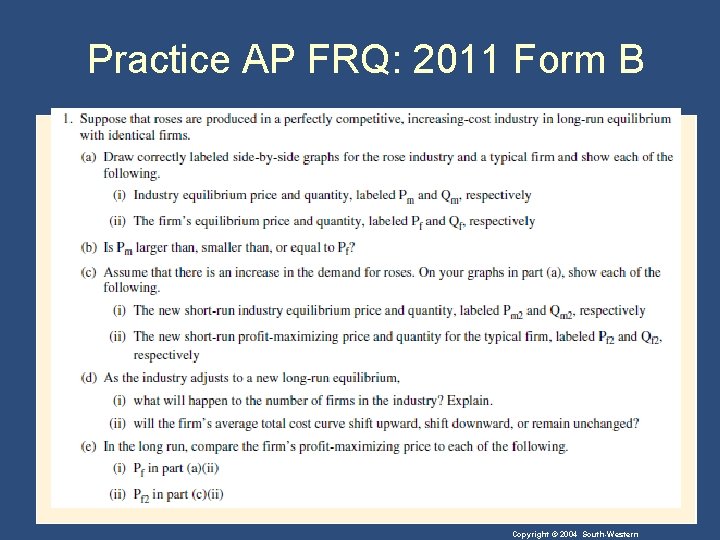
Constant, Increasing, and Decreasing Costs • Perfectly elastic long-run supply is good assumption for many industries; implies constant costs across the industry • • • Some industries have increasing costs; as the industry expands, the price of productive inputs increases due to increased demand for those inputs. • • • Each firm faces the same cost structure; perfectly elastic supply of inputs (i. e. agriculture, bakeries, etc. ) ATC curve does not shift when firms enter or exit the industry ATC curve shifts upwards as more firms enter the industry i. e. beach front resort hotels that must compete for limited quantity of prime beachfront property. Some industries have decreasing costs: as the industry expands, the price of productive inputs decreases due to economies of scale • • ATC curve shifts downwards as more firms entire the industry i. e. electric car industry; economies of scale in the production of lithium batteries lowers input prices • Revisit part (d) and (e) on the 2011 Form B FRQ. How would your responses compare for a firm with constant costs, a firm with increasing costs, and a firm with decreasing costs. Copyright © 2004 South-Western

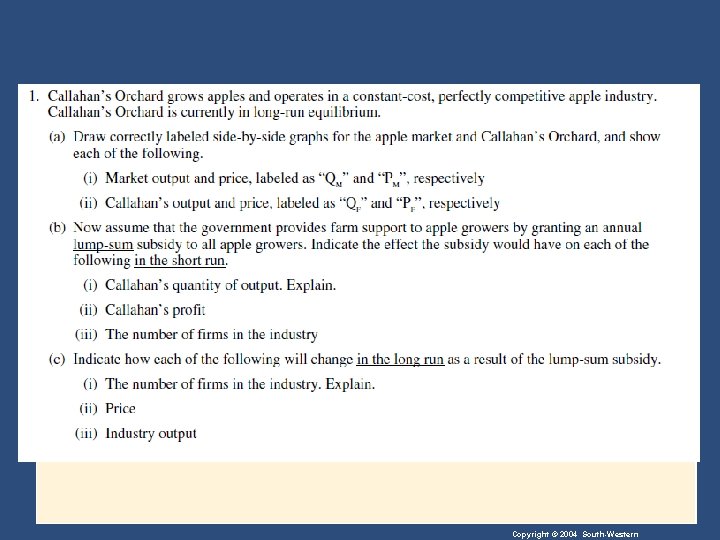
Practice AP FRQ: 2011 Form B Copyright © 2004 South-Western

Copyright © 2004 South-Western

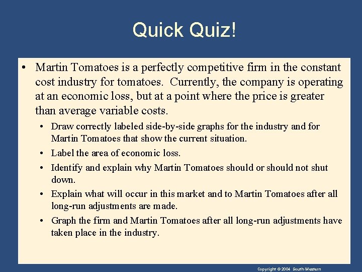
Quick Quiz! • Martin Tomatoes is a perfectly competitive firm in the constant cost industry for tomatoes. Currently, the company is operating at an economic loss, but at a point where the price is greater than average variable costs. • Draw correctly labeled side-by-side graphs for the industry and for Martin Tomatoes that show the current situation. • Label the area of economic loss. • Identify and explain why Martin Tomatoes should or should not shut down. • Explain what will occur in this market and to Martin Tomatoes after all long-run adjustments are made. • Graph the firm and Martin Tomatoes after all long-run adjustments have taken place in the industry. Copyright © 2004 South-Western