Market Structure and Pricing Perfect Competition 1 Firm

Market Structure and Pricing Perfect Competition 1

Firm Decision-Making • In this lecture, we will be focusing on examining how firm’s choose their OUTPUT in order to maximize profits • We will also look at the firm’s decision… – Of how much advertising to conduct (time-depending) • As we will soon see, the firm’s market power (ability to influence price) will depend upon the structure of the market they are in – Are there many other firms competing? – Am I the only firm? – How similar are the products firms produce? 2

Overview • We will talk about three main types of market structure: 1. Perfect Competition 2. Monopoly 3. Oligopoly/Monopolistic Competition 3

Pay Attention… • As we go through the different types of markets, be sure to pay close attention to the assumptions we make • Each type of market structure will have different assumptions and, therefore, different models of behavior • If we want to predict how Pepsi will behave, we need to make sure we are applying the relevant model 4

Perfect Competition 5

Perfectly Competitive Market Structure Characteristics of a Perfectly Competitive Market: 1. 2. 3. 4. Many Buyers and Sellers: each buyer (or seller) is a tiny portion of the total market => no one is very powerful Homogeneous Products: the firms make identical products (agricultural products) Free Entry and Exit: any firm that would like to sell in this industry can and firms are free to exit the industry if they wish (no license requirements, etc. ) Full Information: buyers and sellers are fully informed about the prices and availability of all resources and products 6

Price-Takers • Because each firm is only a small part of the entire market and because the products are homogeneous, we say that firms are price takers (they cannot affect market price) • Why? • The products are identical, so consumers will buy the good with the cheapest price • This market price is established by the supply and demand for the good 7

Some Examples… • Relatively to the other types of market structure, there are not very many examples of perfect competition • Agricultural products (Halloween pumpkins, farmers markets, corn, livestock) • Gold, silver, and copper • Think of foreign currency markets (the market determines the exchange rate) 8

The Use of Perfect Competition • We often refer to perfect competition as the benchmark case for comparing the various types of competition • “How much higher are prices because of monopoly? ” • “How much better off would we (consumers) be if there were more firms offering the product? ” 9

Demand • In our discussion of the perfectly competitive firm, we need to differentiate between market demand the firm’s demand curve • The market demand curve will help us determine the total number of units sold • The firm’s demand curve will help us determine the number of units a particular firm sells • We will illustrate this by looking at the perfectly competitive market for wheat… 10

Horizontal Demand • Because firm’s are price-takers we say that they can sell as many units as they want at the market price • They will not sell anything if they price above the market price • There is no reason to charge below the market price because the firm can sell all that it wants at a higher price • This gives us a horizontal firm demand curve (perfectly elastic demand curve) 11

Market Equilibrium and the Firm’s Demand Curve in Perfect Competition The market price of wheat of $5 per bushel is determined in the left panel by the intersection of the market demand curve and the market supply curve. Once the market price is established, any farmer can sell all he or she wants at that market price. Price per bushel S $5 (b) Firm’s Demand Price per bushel (a) Market Equilibrium d $5 D 0 Bushels of 1, 200, 000 wheat per day 0 5 10 Bushels of 15 wheat per day 12

Short Run Profit Maximization • Because firm’s are price-takers, they have no say in what price will be charged for their good • What CAN they choose? • They can choose how much output to produce at the given market price ☼ The Firm’s Profit Maximizing, then, decision is how much output to produce at the market price ☼ 13

Short-Run Costs and Revenues (1) (2) (3) = (1) (2) (4) Bushels of Marginal Wheat Revenue Total per day (Price) Revenue Cost (q) (p) (TR = q p) (TC) 0 1 2 3 4 5 6 7 8 9 10 11 12 13 14 15 16 -$5 5 5 5 $0 5 10 15 20 25 30 35 40 45 50 55 60 65 70 75 80 $15. 00 19. 75 23. 50 26. 50 29. 00 31. 00 32. 50 33. 75 35. 25 37. 25 40. 00 43. 25 48. 00 54. 50 64. 00 77. 50 96. 00 (5) Marginal Cost MC= TC/ Q -$4. 75 3. 00 2. 50 2. 00 1. 50 1. 25 1. 50 2. 00 2. 75 3. 25 4. 75 6. 50 9. 50 13. 50 18. 50 (6) = (4) + (1) (7) = (3) - (4) Average Total Cost ATC = TC / q Economic Profit or Loss = TR - TC $19. 75 11. 75 8. 83 7. 25 6. 20 5. 42 4. 82 4. 41 4. 14 4. 00 3. 93 4. 00 4. 19 4. 57 5. 17 6. 00 -$15. 00 -14. 75 -13. 50 -11. 50 -9. 00 -6. 00 -2. 50 1. 25 4. 75 7. 75 10. 00 11. 75 12. 00 10. 50 6. 00 -2. 50 -16. 00 14

Alternative Way of Finding Profit Maximizing Output • The profit maximizing level of output occurs where the firm’s marginal revenue (MR) equals its marginal cost (MC) • Marginal Revenue – the change in total revenue from selling an additional unit of output – In perfect competition, the firm’s marginal revenue equals the market price (MR = P) – If the perfectly competitive farmer sells one more pumpkin, how much does his revenue go up? By the amount of the price 15

Marginal Revenue & Marginal Cost • Why is MR = MC the profit maximizing decision? • If MR is greater than MC, what does it mean? • It means that the firm’s revenue will go up more than their costs if they sell an additional unit – Since MR > MC, the firm should expand output • If MR is less than MC, it means that the firm’s revenue will increase by less than their costs if they sell an additional unit – Since MR < MC, the firm should reduce output 16

Short-Run Costs and Revenues (1) (2) (3) = (1) (2) (4) Bushels of Marginal Wheat Revenue Total per day (Price) Revenue Cost (q) (p) (TR = q p) (TC) 0 1 2 3 4 5 6 7 8 9 10 11 12 13 14 15 16 -$5 5 5 5 $0 5 10 15 20 25 30 35 40 45 50 55 60 65 70 75 80 $15. 00 19. 75 23. 50 26. 50 29. 00 31. 00 32. 50 33. 75 35. 25 37. 25 40. 00 43. 25 48. 00 54. 50 64. 00 77. 50 96. 00 (5) Marginal Cost MC= TC/ Q -$4. 75 3. 00 2. 50 2. 00 1. 50 1. 25 1. 50 2. 00 2. 75 3. 25 4. 75 6. 50 9. 50 13. 50 18. 50 (6) = (4) + (1) (7) = (3) - (4) Average Economic Total Cost Profit or ATC = TC / q Loss = TR - TC $19. 75 11. 75 8. 83 7. 25 6. 20 5. 42 4. 82 4. 41 4. 14 4. 00 3. 93 4. 00 4. 19 4. 57 5. 17 6. 00 -$15. 00 -14. 75 -13. 50 -11. 50 -9. 00 -6. 00 -2. 50 1. 25 4. 75 7. 75 10. 00 11. 75 12. 00 10. 50 6. 00 -2. 50 -16. 00 Marginal revenue exceeds marginal cost for the first 12 bushels of wheat. The farmer, as a profit-maximizer will limit output to 12 bushels per day. 17

Short-Run Profit Maximization The marginal cost curve intersects the marginal revenue curve at point e where output is 12 bushels per day. (b) Marginal Cost Equals Marginal Revenue Profit appears in the blue shaded rectangle. The height of the rectangle, ae, equals the price of $5 minus the average cost of $4 per unit profit of $1 per bushel. Marginal cost Average total cost e d = Marginal revenue = average revenue Profit a Dollars per unit At rates of output less than 12 bushels, marginal revenue exceeds marginal cost firm can increase profit by expanding output. At higher rates of output, $5 marginal cost exceeds marginal revenue the firm could 4 increase profit by reducing output. 0 5 10 12 15 Bushels of wheat per day 18

Short-Run Profit Maximization (a) Total Revenue Minus Total Cost The total cost curve shows first increasing then diminishing marginal returns from the variable resource. Total cost Total revenue (= $5 × q ) $60 Total revenue exceeds total cost between 7 and 14 bushels per day economic profit is maximized at the rate of output of 12 bushels of wheat per day. Maximum economic profit = $12 48 Total dollars At output less than 7 bushels and greater than 14 bushels, total cost exceeds total revenue economic loss measured by the vertical distance between the two curves. 15 0 5 7 10 12 15 Bushels of wheat per day Note: At an output of 12 units, the distance between 19 Total Revenue and Total Cost is greatest

Average Revenue • On Slide 18, you may have noticed something called “average revenue” • Average Revenue (AR) – represents the firm’s revenue per unit • AR = (Total Revenue)/(quantity) • In perfect competition, Market Price = Marginal Revenue = Average Revenue 20

Minimizing Short Run Losses • Sometimes the price that the firm is required to “take” will be so low that no rate of output will yield an economic profit • Faced with losses at all rates of output, the firm has two options: – It can continue to produce output even though they are losing money – Or they can temporarily shut down (output falls to zero) 21

Fixed Cost and Minimizing Losses • Recall that the firm has two types of costs in the short run – Fixed cost – Variable cost • A firm that shuts down in the short run must still pay its fixed costs • But, by producing, a firm’s revenue may more than cover variable cost a firm will produce if the revenue thus generated exceeds the variable cost of production can cover a least a portion of its fixed cost 22

Minimizing Losses (1) (2) (3) = (1) (2) (4) Bushels of Marginal Wheat Revenue Total per day (Price) Revenue Cost (q) (p) (TR = q p) (TC) 0 1 2 3 4 5 6 7 8 9 10 11 12 13 14 15 16 -$3 3 3 3 $0 3 6 9 12 15 18 21 24 27 30 33 36 39 42 45 48 $15. 00 19. 75 23. 50 26. 50 29. 00 31. 00 32. 50 33. 75 35. 25 37. 25 40. 00 43. 25 48. 00 54. 50 64. 00 77. 50 96. 00 (5) Marginal Cost MC= TC/ Q -$4. 75 3. 00 2. 50 2. 00 1. 50 1. 25 1. 50 2. 00 2. 75 3. 25 4. 75 6. 50 9. 50 13. 50 18. 50 (6) = (4) + (1) (7) Average Variable Total Cost ATC = TC /q AVC = TVC / q $19. 75 11. 75 8. 83 7. 25 6. 20 5. 42 4. 82 4. 41 4. 14 4. 00 3. 93 4. 00 4. 19 4. 57 5. 17 6. 00 -$4. 75 4. 25 3. 83 3. 50 3. 20 2. 92 2. 68 2. 53 2. 47 2. 50 2. 57 2. 75 3. 04 3. 50 4. 17 5. 06 (8) = (3) - (4) Economic Profit or Loss = TR - TC -$15. 00 -16. 75 -17. 50 -17. 00 -16. 00 -14. 50 -12. 75 -11. 25 -10. 00 -10. 25 -12. 00 -15. 50 -22. 00 -32. 50 -48. 00 Marginal revenue exceeds marginal cost for the first 12 bushels of wheat. Because of the lower price, total revenue is lower at all rates of output and economic profit has disappeared column (8) Column (8) indicates that the firm’s loss is minimized at $10 per day when 10 bushels are produced the net gain of $5 total cost. Exhibit 5 illustrates this same conclusion graphically. 23

Minimizing Short-Run Losses (a) Total Cost and Total Revenue Total cost Total dollars The firm will produce rather than shut down if marginal revenue equals marginal cost at a rate of output where the price equals or exceeds average variable cost. Total revenue (= $3 × q ) $40 30 15 0 5 10 15 Bushels of wheat per day b) Marginal Cost Equals Marginal Revenue Marginal cost Dollars per bushel MR intersects MC at point e, where the output rate is 10 bushels per day and the price of $3 exceeds the average variable cost per bushel of $2. 50. The total economic loss is shown by the shaded area. Minimum economic loss = $10 Average total cost $4. 00 3. 00 2. 50 0 Average variable cost Loss 5 e 10 d = Marginal revenue = average revenue 15 Bushels of wheat per 24 day

Should the Firm Shutdown? • We just looked at the case of a perfectly competitive firm losing money in the short run • As long as the loss that results from producing is less than the shutdown loss, the firm will remain open for business in the short run • However, if the average variable cost of production exceeds the price of all rates of output, the firm will shut down • Shut down vs. Going out of Business 25

Short Run Supply Curves • Now we will look at how to find the firm’s supply curve • Using the supply curve for each firm, we will then find the market supply curve (similar to finding market demand curves) • To begin thinking about how to construct the firm supply curve, think about how much output the firm would produce at every price level 26

Dollars per unit Marginal cost 5 p 5 4 p 4 3 p 3 2 p 1 d 5 d 4 Average variable cost d 3 d 2 d 1 1 Shutdown point 0 q q q 3 q q 1 2 Quantity period 4 5 27

Short-Run Firm Supply Curve • As long as the price covers average variable cost, the firm will supply the quantity resulting from the intersection of its upward-sloping marginal cost curve and its marginal revenue, or demand curve • Thus, that portion of the firm’s marginal cost curve that intersects and rises above the lowest point on its average variable cost curve becomes the short-run firm supply curve 28

Short Run Industry Supply Curve • In order to find the industry supply curve we horizontally sum all of the individual firm supply curves • The process is very similar to what we did when finding the market demand curve based on individual demand curves • At each price level, we will add up the output that each firm is willing to supply 29

Aggregating Individual Supply to Form Market Supply Price per unit (a) Firm A (b) Firm B SA (d) Industry, or market, supply (c) Firm C SA + SC SB p' p' p p 0 10 20 Quantity per period 0 10 20 Quantity period 0 30 SB + SC = S 60 Quantity period The short-run industry supply curve is the horizontal sum of all firms’ short-run supply curves horizontal summation of the firm level marginal cost curves At a price below p, no output is supplied. At a price of p, each of the three firms supplies 10 units, for a market supply of 30 units, and at a price of p', each firm supplies 20 units the market supply is 60 units. 30

Perfect Competition in the Long Run • Once again, we need to distinguish between the short run and the long run • In the short run, a firm takes the market price as given and chooses the quantity of output that maximizes profit (P=MR=MC) • This firm can earn a profit or a loss • If losing money, the firm decides whether to continue operating or shutdown • In the long run, things are a little different… 31

Perfect Competition in the Long Run • In the long run, recall that there is free entry & exit of firms and resources… • Short Run Profit leads to entry as this industry appears attractive to other firms • Short Run Loss leads to exit as firms either reduce the scale of their operations or they exit the industry to engage in something more profitable • The Result? • Zero Profit in the Long Run 32

Zero Profit in the Long Run • This “zero profit” is equivalent to saying “normal profit” • We will now look at how this transition to zero profit occurs in the long run • The key element will be the change in market supply caused by entry and exit • Exit => reduces the market supply • Entry => increases the market supply 33

S MC ATC D P* P* D q* Q* • The market supply and demand determine the market price • P = MC (or MR = MC) determines the firm’s level of output (q*) • At the profit maximizing level of output, the price is greater than the average total cost (or the cost per unit) • The firm, therefore, earns profit • In the long run, the profit leads to ENTRY… 34

S MC S’ ATC P* D P’ D’ P* P’ D q’ q* Q* Q’ • The ENTRY leads to an increase in the number of firms, which shifts OUT the supply curve • This leads to a LOWER equilibrium price • At P’, the firm selects output be equating MC and Price • The result, however, is zero profit because P = ATC 35

Long Run Rule • In the long run, firms (again) choose their level of output by equating P = MR = MC • The firm earns zero profit in the long run • P = MR = MC = ATC • The amount the firm receives (per unit) is actually equal to the cost (per unit) • We just examined the case where the firm earns short run profit • On your own, try and draw the case where the firm is losing money in the short run 36

Perfect Competition and Efficiency • As I have already said, perfect competition will often serve as our benchmark • Why? • Because perfect competition is the most efficient market structure • In economics, we measure efficiency using: – Productive Efficiency – Allocative Efficiency 37

Economic Efficiency • Productive Efficiency – producing output at the least possible cost • Allocative Efficiency – producing the output that consumers value the most • Perfect competition yields both productive and allocative efficiency in the long run 38

Productive Efficiency • Productive efficiency implies that output is produced at the lowest possible cost • Graphically, this means that production should occur at the bottom of the average total cost curve • If you look back at the Long Run graphs, you’ll notice that zero profit occurs where Price equals Average Total Cost ATC P’ D = MR 39

Allocative Efficiency • Producing “what consumers want” requires that the marginal benefit from the good equals the marginal cost • Recall that the demand curve tells us what consumers are willing to pay for the good • Under perfect competition, the last unit consumers buy is “worth” exactly what they pay => this is allocative efficiency • Recall the examples of consumer surplus 40

How Do We Measure How “Good” Perfect Competition Is? • We will use Total Suplus, which is Consumer Surplus Producer Surplus • TS = CS + PS • Consumer Surplus – the difference between what a consumer is willing to pay for a unit of a good and what they actually pay for the unit • Producer Surplus – the difference between the price a producer is willing to provide at and the price they actually receive (similar to profit) – Similar to consumer surplus 41

Consumer Surplus and Producer Surplus Consumer surplus is shown by the blue shaded area, which is the area below the demand curve but above the market clearing price of $10. Producers also derive a net benefit, or a surplus, from market exchange because the amount they receive for their output exceeds the minimum amount they would require to supply that $10 amount in the short run. Recall that the short-run market 5 supply curve is the sum of that portion of each firm’s marginal cost curve at or above the minimum point on its average variable cost curve point m on 0 the market supply curve S. Dollars per unit Consumer surplus S e Producer surplus D m Quantity period 100, 000 120, 000 200, 000 42

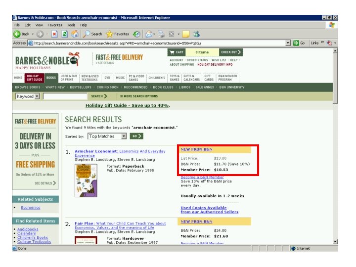
Does the Internet Lead to Perfect Competition? • Many economists have wondered whether the internet will/has lead to perfect competition • Why? • The internet makes it easy to search for the best price • For example, suppose I am interested in buying an i. Pod MP 3 player from Apple • A number of places are available online to purchase an i. Pod… 43

The Internet and Perf. Comp • Shouldn’t we get the same price from every store online? • Homogeneous Products – all of the stores sell the same Apple i. Pod mp 3 player (no store’s i. Pod is “better” than any others) • Number of Sellers – there are tons of online stores (Best. Buy, Circuit City, Amazon, etc. ) • Free Entry and Exit – it’s very low cost to start a website, no prohibitions or legal restrictions • Full Information – the internet has made it very easy to search for the best price (consumers and firms are fully informed about 44 the market price)

But… • We haven’t yet seen perfect competition in on the online market for goods • Prices are not the same for all firms (websites) • Consider the following results when I used www. shopping. com to search for the best i. Pod prices… 45

46

Price Comparison • Notice the price ranges… • For the 120 GB 6 th Generation i. Pod, the price range was from $170 to $250 • This is for two stores selling the same exact product • Almost all other products have similar price ranges • Has the internet lead to perfect competition? • Why or why not? !? 47

Monopoly

Barriers to Entry • A monopolist is the only producer of a product with no close substitute – “Local monopoly” (market definition) • The key reason that there is only one producer is that there is some barrier to entry • Barrier to entry – something that impedes other firms from entering the industry – Legal restrictions – Economies of scale – Control of essential (natural) resources

Legal Restrictions • Patents, licenses, and other legal restrictions (imposed by the government or some governing body) provide some producers legal protection from competition • Patents – a way to protect inventors (innovators) from having their creations “stolen” by other firms or people • Licenses – when the government grants the exclusive right to supply a particular good or service • Some examples…

Examples… • New Era Cap Company is the “exclusive supplier” of hats for Major League Baseball teams • Reebok is the official supplier of NFL jerseys • According to the Gillette website, the Gillette M 3 Power razor is protected by 62 patents • Local examples: GT&T (land line phone service), Guysuco, GWI, GPL, UG (effectively), the companies that operate the Berbice and Demerara Harbour Bridges, GPO (effectively), GDF, NCN – Radio, …

Economies of Scale • A single firm can sometimes satisfy market demand at a lower average cost of production than two or three firms could • In other words, one big firm can provide the good cheaper than several smaller firms can • This is usually true for firms or industries where average total cost falls as output increases • Economies of scale can be a reason FOR legal restrictions • Examples…(utilities)

Examples… • GT&T is the only local land-line telephone service that I can receive because of the scale economies present • Electricity generation and distribution (GPL) – Note that in many countries, the generation of electricity is fairly competitive

Road Map for Monopoly 1. Profit Maximizing choices of output and/or price 2. Comparing monopoly with perfect competition 3. More “creative” pricing strategies: 1. Price Discrimination 2. Two-part Pricing

Revenue for the Monopolist • When dealing with a monopolist, it is no longer necessary to distinguish between a firm’s demand curve and the market demand curve • Why? • Because the monopolist is the only firm serving the market, so the market demand curve is the firm’s demand curve • The monopolist, therefore, faces a downward sloping demand curve for his or her product

Demand Marginal Revenue • Let’s consider the example of GT&T’s land line phone service • GT&T has been granted a license by the government to be the sole land line provider operating in Guyana • GT&T has (say) 300, 000 subscribers at a price of (say) $100 per month for rental of the lines • Their TOTAL REVENUE from rental is $30, 000

Demand Marginal Revenue • Suppose that in order to increase the number of subscribers to 400, 000, GT&T would have to lower the rental price to $67. 60 per month • Even though GT&T is a monopolist, it are still constrained by the law of demand • GT&T’s new TOTAL REVENUE would be $27, 040, 000 • What is the marginal revenue from selling one more unit?

Demand Marginal Revenue • Under perfect competition, the firm’s marginal revenue was simply the price (because they could sell as many units as they wanted at the market price) • For a monopolist, marginal revenue does NOT equal the price • Why? • In order to sell an additional unit, you need to lower your price

Demand Marginal Revenue • Mathematically, what is marginal revenue? • Marginal Revenue – the change in total revenue divided by the change in output

Calculating Marginal Revenue • So, in our example, Comcast’s Total Revenue went from $30 million to $27, 040, 000 and their sales went from 300, 000 to 400, 000: • The marginal revenue equals $29. 60

Loss or Gain from Selling One More Unit $100 By selling to additional customers, GT&T gains the revenue from selling to more customers than they did before LOSS 67. 60 However, to gain additional customers, GT&T much charge a lower price which means they receive less money per customer Price per month D G A I N 0 3 If the GAIN is greater than the LOSS, then lowering the price increases TOTAL REVENUE and MARGINAL REVENUE IS POSITIVE, and vice versa 4 Customers in ‘ 00, 000

Monopoly Demand Marginal and Total Revenue Note that the marginal revenue curve is below the demand curve and total revenue is at a maximum when marginal revenue equals zero. Dollars per month (a) Demand Marginal Revenue Demand marginal revenue are shown in the upper panel and total revenue is in the lower panel. Elastic Unit elastic $37. 50 Inelastic 0 D = Average revenue Marginal revenue 16 Millions of customers (b) Total Revenue $600 million Total dollars Notice also that when demand is elastic, a decrease in price increases total revenue marginal revenue is positive. Conversely, when demand is inelastic, a decrease in price reduces total revenue marginal revenue is negative 32 Total revenue 0 16 32 Millions of customers

Profit Maximization • In perfect competition, firm’s were not able to select their price…instead they chose the optimal level of output • A monopolist, on the other hand, can choose either the price or quantity in order to maximize profit • Because the monopolist is constrained by the demand curve, choosing one things automatically tells you the value of the other choice • Because the monopolist can set price, we say that it has some market power

Profit Maximization • To illustrate how the monopolist chooses her optimal price (or quantity), consider the following data for De Beers We will combine cost data with information on their total revenue in order to determine the profit maximizing price/quantity • As you will see, the monopolist (much like the perfectly competitive firm) will choose to produce where MARGINAL COST EQUALS MARGINAL REVENUE

Short-Run Revenues and Costs for the Monopolist Short-run Costs and Revenue for a Monopolist Diamonds per day (Q) (1) 0 1 2 3 4 5 6 7 8 9 10 11 12 13 14 15 16 17 Price Marginal (average Total Revenue revenue) revenue (MR = (p) (TR = Q x p) TR / Q) (2) (3) =(1) x (2) (4) $7, 750 7, 500 7, 250 7, 000 6, 750 6, 500 6, 250 6, 000 5, 750 5, 500 5, 250 5, 000 4, 750 4, 500 4, 250 4, 000 3, 750 3, 500 0 $7, 500 14, 500 21, 000 27, 000 32, 500 37, 500 42, 000 46, 000 49, 500 52, 500 55, 000 57, 000 58, 500 59, 500 60, 000 59, 500 $7, 500 7, 000 6, 500 6, 000 5, 500 5, 000 4, 500 4, 000 3, 500 3, 000 2, 500 2, 000 1, 500 1, 000 500 0 -500 Marginal Average Total Cost Profit or Cost ( MC = (ACT = Loss = (TC) TC / Q) TC/Q) TR - TC (5) (6) (7) (8) $15, 000 19, 750 23, 500 26, 500 29, 000 31, 000 32, 500 33, 750 35, 250 37, 250 40, 000 43, 250 48, 000 54, 500 64, 000 77, 500 96, 000 121, 000 4, 750 3, 000 2, 500 2, 000 1, 500 1, 250 1, 500 2, 000 2, 750 3, 250 4, 750 6, 500 9, 500 13, 500 18, 500 25, 000 -$15, 000 $19, 750 -12, 250 11, 750 9, 000 8, 830 -5, 500 7, 750 -2, 000 6, 200 1, 500 5, 420 5, 000 4, 820 8, 250 4, 410 10, 750 4, 140 12, 250 4, 000 12, 500 3, 930 11, 750 4, 000 9, 000 4, 190 4, 000 4, 570 -4, 500 5, 170 -7, 500 6, 000 -36, 000 7, 120 -61, 500 The profitmaximizing monopolist employs the same decision rule as the competitive firm the monopolist produces that quantity where total revenue exceeds total cost by the greatest amount $12, 500 per day when output is 10 units per day. Total revenue is $52, 500 and total cost is $40, 000

Profit Maximization Graphically Price per diamond Marginal Cost $5, 250 Average Total Cost $4, 000 MR 10 16 Demand 32 Diamonds per day • The monopolist chooses the level of output by equating marginal cost and marginal revenue • But the price comes from the DEMAND CURVE

Short Run Losses • I have just drawn the case where the monopolist is earning profit in the short run • A monopolist is not guaranteed profit, however • Being a monopolist does not guarantee profit because the monopolist is still constrained by the demand for the product

Short Run Losses • If a monopolist is losing money in the short run, the firm must make the decision that a perfectly competitive firm does: – Should I continue to operate even though I’m losing money? – Or should I temporary suspend operations? • The decision depends on which strategy is more effective in minimizing losses

Long Run Profit Maximization • The distinction between the short run and long run is not as important under monopoly • Barriers to entry provide some protection for the monopolist and allow for the possibility of long run profit – Recall how free entry and exit eliminated profit in the long run • The primary difference between the short run and the long run is that the monopolist may adjust the size (or scale) of the firm to more efficiently serve the market

Monopoly vs. Perfect Competition • We will now compare the price level and amount of output for a monopolist versus the outcome we would’ve had under perfect competition • Keep in mind the “profit-maximizing rules” – Perfect Competition: P = MC – Monopoly: MR = MC (and price comes from the demand curve) • Let’s look at a simple picture…

Perfect Competition and Monopoly yield price pc and quantity Qc. The monopolist maximizes profit by equating marginal revenue with marginal cost point b equilibrium price pm and output Qm. a Dollars per unit Equilibrium in perfect competition is at point c, where market demand the marginal cost curve intersect to m p' m c pc b MC D MRm 0 Q'm Qc Quantity period Consumer surplus under MONOPOLY is the yellow triangle. Consumer surplus under PERFECT COMPETITION is the checkered green triangle NOTE: The green triangle INCLUDES the yellow triangle Consumer surplus under PERFECT COMPETITION is clearly LARGER

Welfare Under Monopoly • There are several reasons to think that the welfare measure we have used might understate or overstate the welfare loss due to monopoly • Reasons the Welfare Loss May Be Lower: – Economies of scale could make production very cheap – The monopolist may under-price because of government regulation or public scrutiny – Monopolies may under-price in order to keep potential competitors out (make it less attractive) • Reasons the Welfare Loss May Be Greater: – Monopolies spend a lot of money in order to protect their product (lawyers, advertising, market research) – Monopolies may be slow to adopt new technology which would benefit the consumer (no competition…why do I need to make the product better? )

Pricing with Market Power • When firms use a single per-unit uniform price (like we have just looked at), this leave consumers with consumer surplus • The desire to capture some of this consumer surplus leads firms to adopt more “creative” pricing strategies • Here are some examples…

Price Discrimination • Price discrimination – charging different prices for the same product • The fundamental idea: firms believe that different groups (or “types”) of individuals have different demands for the product – The firm then charges each group/type a price that is appropriate given their demand • Three degrees of price discrimination

Examples… • The key to all of these examples is that they represent times when the firm is charging different prices for the same product • Movie tickets: Senior Citizens & Children vs. Adults • Haircuts: Women pay more than men • Airfare: Business travelers vs. Leisure travelers • Cell phone plans: choosing the number of night and weekend minutes vs. anytime minutes • Buying things in “bulk”…

Price Discrimination (b) Dollars per unit (a) $3. 00 MC 1. 00 MR 0 400 $1. 50 1. 00 D Quantity period 0 MC D' MR' 500 Quantity period Consumer #1 (the left hand side) has a more inelastic demand for the product than Consumer #2 (the right hand side). To exploit this difference the monopolist charges separate prices to each consumer. This strategy yields the monopolist more profit than simply charging a “uniform” price to both consumers.

Two-Part Pricing • Two-part pricing refers to a strategy where the firm charges a price per unit and a fee that does not depend on the usage • The goal is to use the fee to “steal” some of the consumer surplus that is leftover • Examples: – Telephone – Amusement parks – Dance clubs & Bars

How it works… • Whenever there is consumer surplus, it means that the consumer was willing to pay more than he did… • My favorite band puts out a new CD and I would be willing to pay $40 for it • The store only charges $15, so I get a benefit (consumer surplus) of $25 • If the store charged $15 for the CD plus $25 as a membership fee, I would still be willing to buy the CD ($15 + $15 = $30), but now the firm receives a higher profit

Required Tie-In Sales • Bundling is sometimes also referred to as a “tie-in” sale • The consumer, however, has the option to purchase either OR both of the goods • In required tie-in sales, the consumer is required to purchase both goods (you cannot buy one separately) • Examples – – Mach 3 Turbo razor vs. Schick Quattro Sony Playstation 2 vs. Microsoft X-Box Polaroid instant camera Photocopiers (Xerox)

Peak-Load Pricing • Charging a higher price during peak times (i. e. high demand times) • Examples: – Electricity pricing (the price per kilowatt hour changes depending on what time of day…so do you laundry at midnight) – Rental properties (renting a place in Destin is pretty cheap in January) – Car Rentals (the price of car rentals is higher during the summer…vacation season) – Matinee vs. Regular Admission (movie theaters charge lower prices during the day…lower demand period)