Part II Sigma Freud Descriptive Statistics Chapter 3

Part II Sigma Freud & Descriptive Statistics Chapter 3 Viva La Difference: Understanding Variability

What you will learn in Chapter 3 • Variability is valuable as a descriptive tool • Difference between variance & standard • deviation How to compute: • Range • Inter-quartile Range • Standard Deviation • Variance

Why Variability is Important l Variability • how different scores are from one particular score • Spread • Dispersion l l What is the “score” of interest here? • Ah ha!! It’s the MEAN!! So…variability is really a measure of how each score in a group of scores differs from the mean of that set of scores.

l Measures of Variability Four types of variability that examine the amount of spread or dispersion in a group of scores… • Range • Inter-quartile Range • Standard Deviation • Variance l Typically report the average and the variability together to describe a distribution.

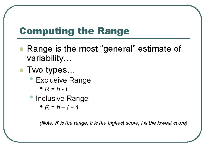
Computing the Range l l Range is the most “general” estimate of variability… Two types… • Exclusive Range • R=h-l • Inclusive Range • R=h–l+1 (Note: R is the range, h is the highest score, l is the lowest score)

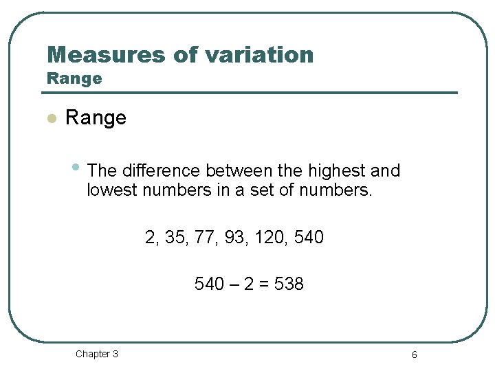
Measures of variation Range l Range • The difference between the highest and lowest numbers in a set of numbers. 2, 35, 77, 93, 120, 540 – 2 = 538 Chapter 3 6

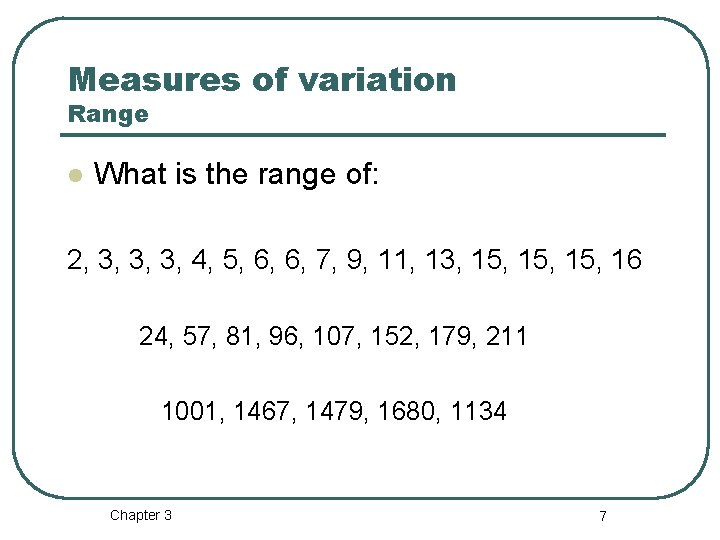
Measures of variation Range l What is the range of: 2, 3, 3, 3, 4, 5, 6, 6, 7, 9, 11, 13, 15, 15, 16 24, 57, 81, 96, 107, 152, 179, 211 1001, 1467, 1479, 1680, 1134 Chapter 3 7

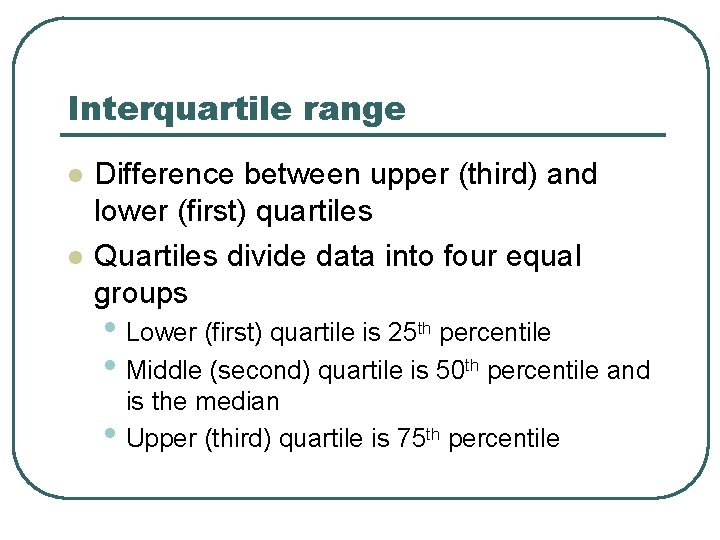
Interquartile range l l Difference between upper (third) and lower (first) quartiles Quartiles divide data into four equal groups • Lower (first) quartile is 25 th percentile • Middle (second) quartile is 50 th percentile and • is the median Upper (third) quartile is 75 th percentile

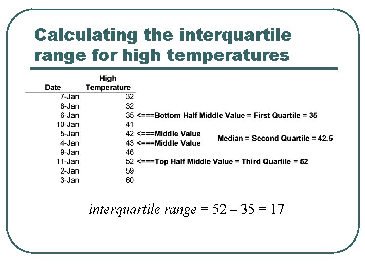
Calculating the interquartile range for high temperatures interquartile range = 52 – 35 = 17

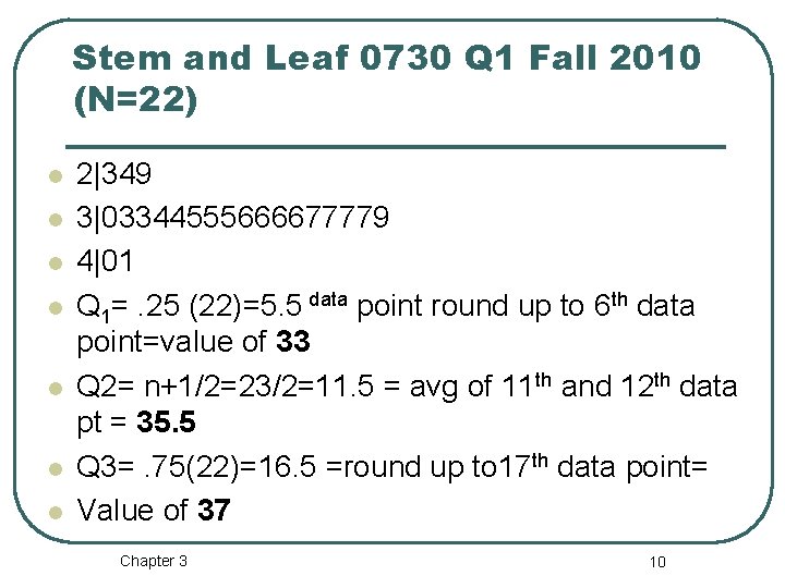
Stem and Leaf 0730 Q 1 Fall 2010 (N=22) l l l l 2|349 3|03344555666677779 4|01 Q 1=. 25 (22)=5. 5 data point round up to 6 th data point=value of 33 Q 2= n+1/2=23/2=11. 5 = avg of 11 th and 12 th data pt = 35. 5 Q 3=. 75(22)=16. 5 =round up to 17 th data point= Value of 37 Chapter 3 10

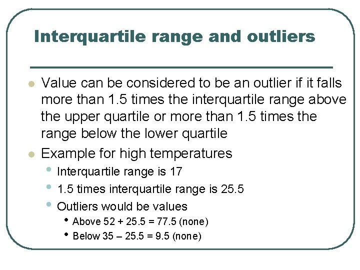
Interquartile range and outliers l l Value can be considered to be an outlier if it falls more than 1. 5 times the interquartile range above the upper quartile or more than 1. 5 times the range below the lower quartile Example for high temperatures • Interquartile range is 17 • 1. 5 times interquartile range is 25. 5 • Outliers would be values • Above 52 + 25. 5 = 77. 5 (none) • Below 35 – 25. 5 = 9. 5 (none)

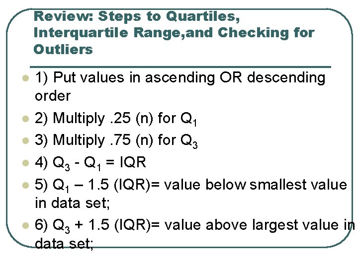
Review: Steps to Quartiles, Interquartile Range, and Checking for Outliers l l l 1) Put values in ascending OR descending order 2) Multiply. 25 (n) for Q 1 3) Multiply. 75 (n) for Q 3 4) Q 3 - Q 1 = IQR 5) Q 1 – 1. 5 (IQR)= value below smallest value in data set; 6) Q 3 + 1. 5 (IQR)= value above largest value in data set;

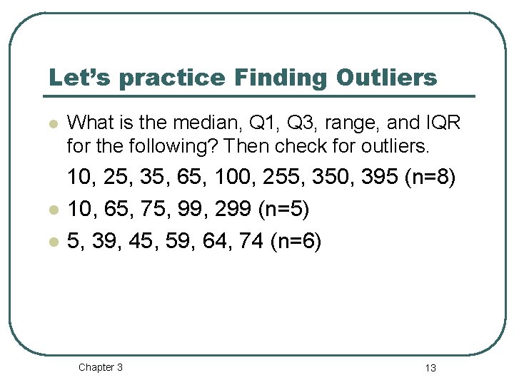
Let’s practice Finding Outliers l What is the median, Q 1, Q 3, range, and IQR for the following? Then check for outliers. 10, 25, 35, 65, 100, 255, 350, 395 (n=8) l 10, 65, 75, 99, 299 (n=5) l 5, 39, 45, 59, 64, 74 (n=6) Chapter 3 13

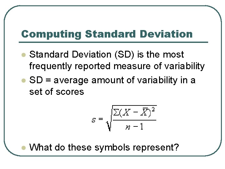
Computing Standard Deviation l l l Standard Deviation (SD) is the most frequently reported measure of variability SD = average amount of variability in a set of scores What do these symbols represent?

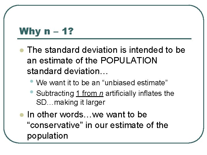
Why n – 1? l The standard deviation is intended to be an estimate of the POPULATION standard deviation… • We want it to be an “unbiased estimate” • Subtracting 1 from n artificially inflates the SD…making it larger l In other words…we want to be “conservative” in our estimate of the population

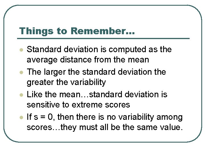
Things to Remember… l l Standard deviation is computed as the average distance from the mean The larger the standard deviation the greater the variability Like the mean…standard deviation is sensitive to extreme scores If s = 0, then there is no variability among scores…they must all be the same value.

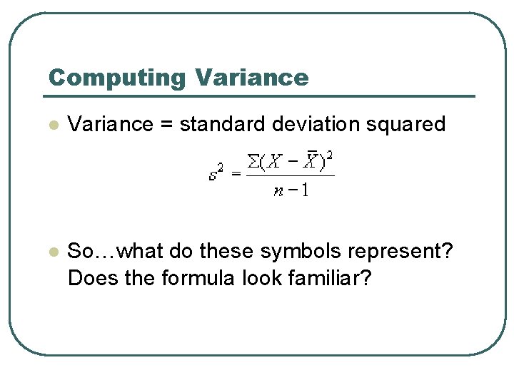
Computing Variance l Variance = standard deviation squared l So…what do these symbols represent? Does the formula look familiar?

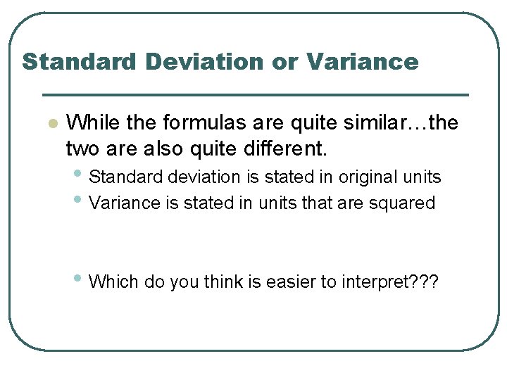
Standard Deviation or Variance l While the formulas are quite similar…the two are also quite different. • Standard deviation is stated in original units • Variance is stated in units that are squared • Which do you think is easier to interpret? ? ?

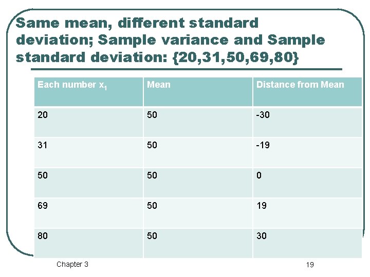
Same mean, different standard deviation; Sample variance and Sample standard deviation: {20, 31, 50, 69, 80} Each number x 1 Mean Distance from Mean 20 50 -30 31 50 -19 50 50 0 69 50 19 80 50 30 Chapter 3 19

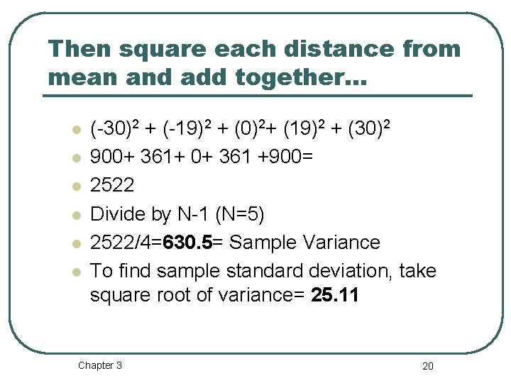
Then square each distance from mean and add together… l l l (-30)2 + (-19)2 + (0)2+ (19)2 + (30)2 900+ 361+ 0+ 361 +900= 2522 Divide by N-1 (N=5) 2522/4=630. 5= Sample Variance To find sample standard deviation, take square root of variance= 25. 11 Chapter 3 20

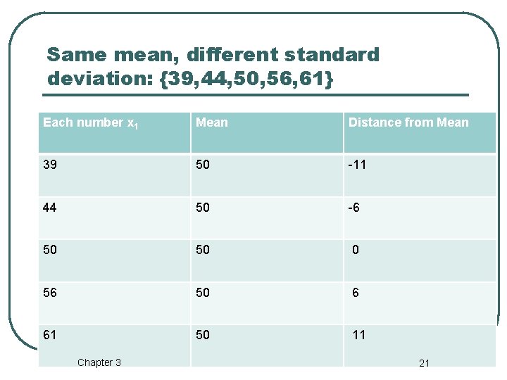
Same mean, different standard deviation: {39, 44, 50, 56, 61} Each number x 1 Mean Distance from Mean 39 50 -11 44 50 -6 50 50 0 56 50 6 61 50 11 Chapter 3 21

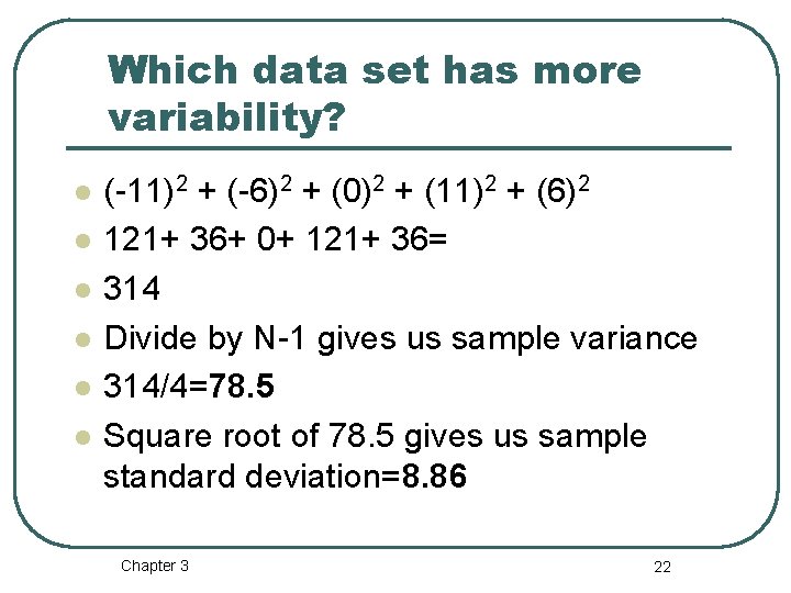
Which data set has more variability? l l l (-11)2 + (-6)2 + (0)2 + (11)2 + (6)2 121+ 36+ 0+ 121+ 36= 314 Divide by N-1 gives us sample variance 314/4=78. 5 Square root of 78. 5 gives us sample standard deviation=8. 86 Chapter 3 22

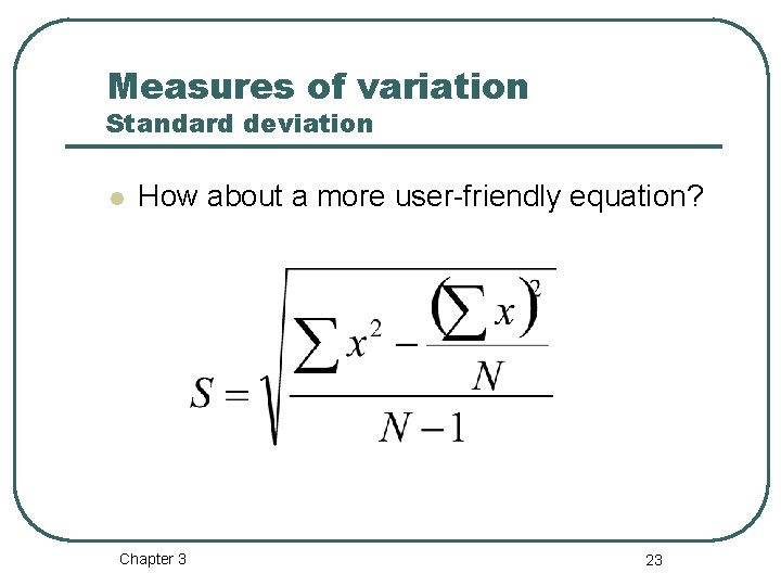
Measures of variation Standard deviation l How about a more user-friendly equation? Chapter 3 23

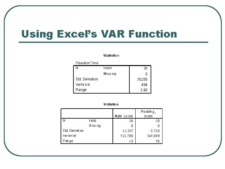
Using Excel’s VAR Function

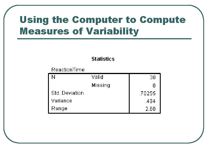
Using the Computer to Compute Measures of Variability

Glossary Terms to Know l Variability • Range • Standard deviation • Mean deviation • Unbiased estimate • Variance