Parameter Learning in MN Outline CRF Learning CRF

Outline • CRF • Learning CRF for 2 -d image segmentation • IPF parameter

Log-linear Markov network (most common representation) • Feature is some function [D] for some

Generative v. Discriminative classifiers – A review • Want to Learn: h: X �Y

Log-linear CRFs (most common representation) • Graph H: only over hidden vars Y 1,

Example: Image Segmentation - A set of features 1[D 1], …, k[Dk] – each

Example: Image Segmentation y 1 y 2 y 3 y 4 y 5 y

Example: Inference for Learning How to compute E[Cfb|X[n]] y 1 y 2 y 3

Representation Equivalence Log linear representation Tabular MN representation from HW 4 y 1 y

Tabular MN representation from HW 4 Now do it over the edge potential This

Iterative Proportional Fitting (IPF) Coherence Difficulty Intelligence • Setting derivative to zero: Grade SAT

Parameter Sharing in your HW • Note that I am suing Y for label

IPF parameter sharing We only have one data point (image) in this example so

Slides: 20

Download presentation

Parameter Learning in MN

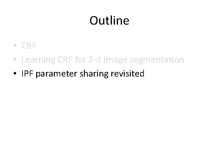
Outline • CRF • Learning CRF for 2 -d image segmentation • IPF parameter sharing revisited

Log-linear Markov network (most common representation) • Feature is some function [D] for some subset of variables D – e. g. , indicator function • Log-linear model over a Markov network H: – a set of features 1[D 1], …, k[Dk] • each Di is a subset of a clique in H • two ’s can be over the same variables – a set of weights w 1, …, wk • usually learned from data – 10 -708 – �Carlos Guestrin 2006 -2008 3

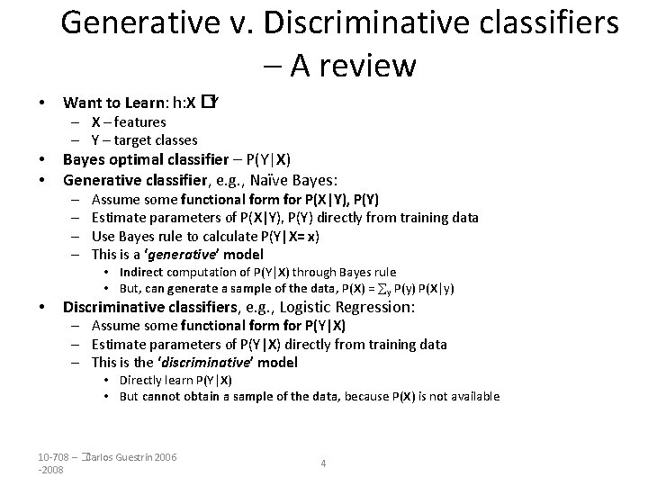
Generative v. Discriminative classifiers – A review • Want to Learn: h: X �Y – X – features – Y – target classes • • Bayes optimal classifier – P(Y|X) Generative classifier, e. g. , Naïve Bayes: – – • Assume some functional form for P(X|Y), P(Y) Estimate parameters of P(X|Y), P(Y) directly from training data Use Bayes rule to calculate P(Y|X= x) This is a ‘generative’ model • Indirect computation of P(Y|X) through Bayes rule • But, can generate a sample of the data, P(X) = y P(y) P(X|y) Discriminative classifiers, e. g. , Logistic Regression: – Assume some functional form for P(Y|X) – Estimate parameters of P(Y|X) directly from training data – This is the ‘discriminative’ model • Directly learn P(Y|X) • But cannot obtain a sample of the data, because P(X) is not available 10 -708 – �Carlos Guestrin 2006 -2008 4

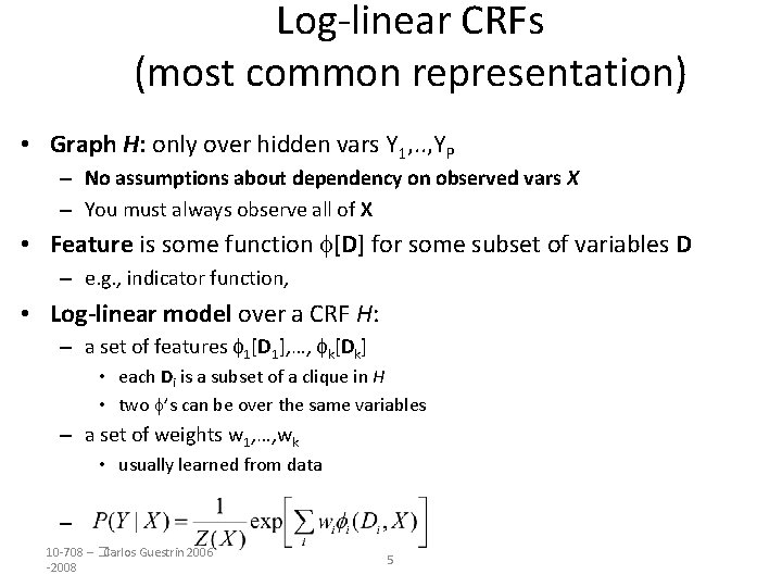
Log-linear CRFs (most common representation) • Graph H: only over hidden vars Y 1, . . , YP – No assumptions about dependency on observed vars X – You must always observe all of X • Feature is some function [D] for some subset of variables D – e. g. , indicator function, • Log-linear model over a CRF H: – a set of features 1[D 1], …, k[Dk] • each Di is a subset of a clique in H • two ’s can be over the same variables – a set of weights w 1, …, wk • usually learned from data – 10 -708 – �Carlos Guestrin 2006 -2008 5

Example: Image Segmentation - A set of features 1[D 1], …, k[Dk] – each Di is a subset of a clique in H – two ’s can be over the same y 1 y 2 y 3 y 4 y 5 y 6 y 7 y 8 y 9 variables We will define features as follows: : measures compatibility of node color and its segmentation - A set of indicator features triggered for each edge labeling pair {ff, bb, fb, bf} - This is a allowed since we can define many features overr the same subset of variables

Example: Image Segmentation - A set of features 1[D 1], …, k[Dk] – each Di is a subset of a clique in H – two ’s can be over the same y 1 y 2 y 3 y 4 y 5 y 6 y 7 y 8 y 9 variables

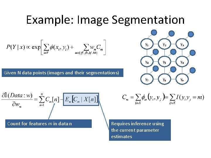
Example: Image Segmentation - A set of features 1[D 1], …, k[Dk] – each Di is a subset of a clique in H – two ’s can be over the same variables -Now we just need to sum these features We need to learn parameters wm y 1 y 2 y 3 y 4 y 5 y 6 y 7 y 8 y 9

Example: Image Segmentation y 1 y 2 y 3 y 4 y 5 y 6 y 7 y 8 y 9 Given N data points (images and their segmentations) Count for features m in data n Requires inference using the current parameter estimates

Example: Inference for Learning How to compute E[Cfb|X[n]] y 1 y 2 y 3 y 4 y 5 y 6 y 7 y 8 y 9

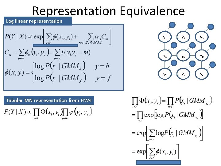
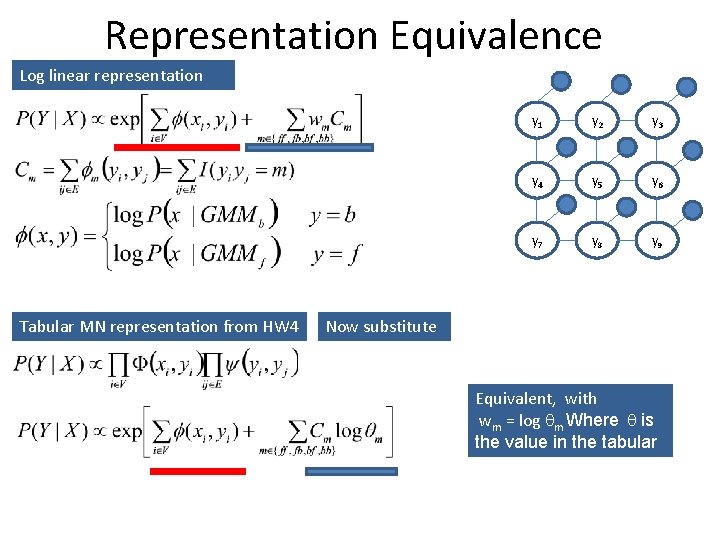
Representation Equivalence Log linear representation Tabular MN representation from HW 4 y 1 y 2 y 3 y 4 y 5 y 6 y 7 y 8 y 9

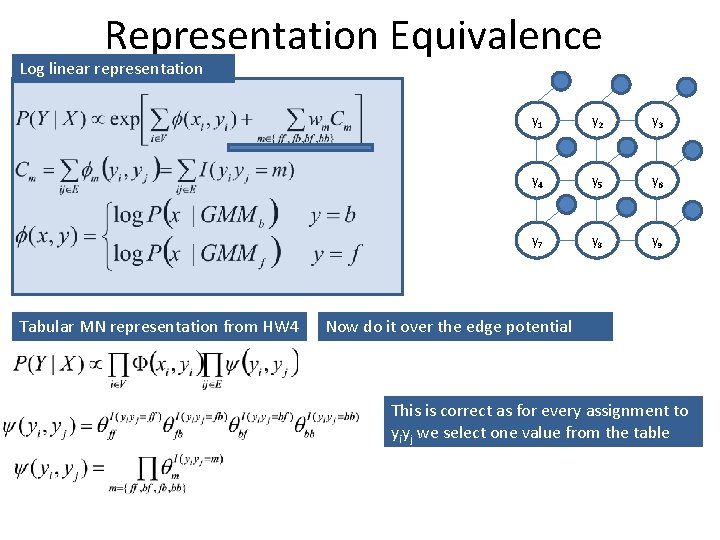
Representation Equivalence Log linear representation Tabular MN representation from HW 4 y 1 y 2 y 3 y 4 y 5 y 6 y 7 y 8 y 9 Now do it over the edge potential This is correct as for every assignment to yiyj we select one value from the table

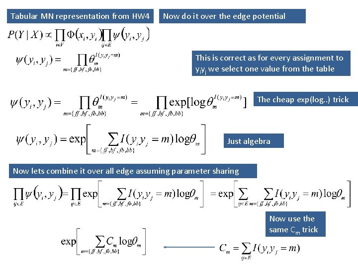
Tabular MN representation from HW 4 Now do it over the edge potential This is correct as for every assignment to yiyj we select one value from the table The cheap exp(log. . ) trick Just algebra Now lets combine it over all edge assuming parameter sharing Now use the same Cm trick

Representation Equivalence Log linear representation Tabular MN representation from HW 4 y 1 y 2 y 3 y 4 y 5 y 6 y 7 y 8 y 9 Now substitute Equivalent, with wm = log qm Where q is the value in the tabular

Outline • CRF • Learning CRF for 2 -d image segmentation • IPF parameter sharing revisited

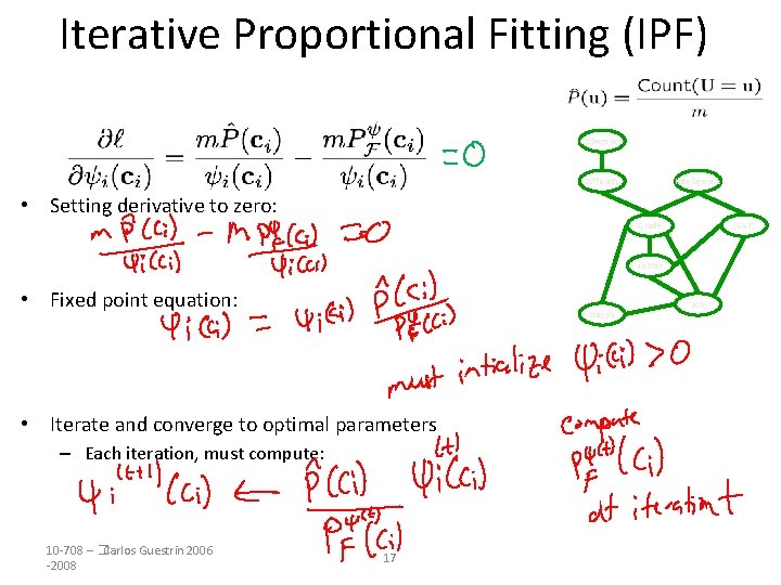
Iterative Proportional Fitting (IPF) Coherence Difficulty Intelligence • Setting derivative to zero: Grade SAT Letter • Fixed point equation: Happy • Iterate and converge to optimal parameters – Each iteration, must compute: 10 -708 – �Carlos Guestrin 2006 -2008 17 Job

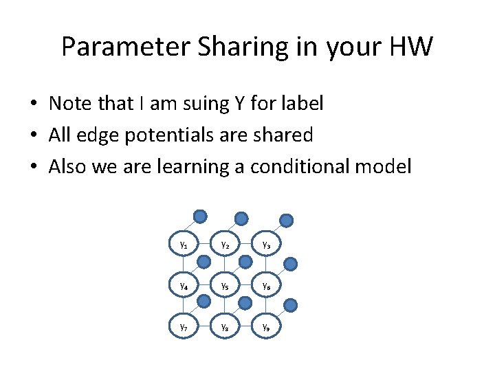
Parameter Sharing in your HW • Note that I am suing Y for label • All edge potentials are shared • Also we are learning a conditional model y 1 y 2 y 3 y 4 y 5 y 6 y 7 y 8 y 9

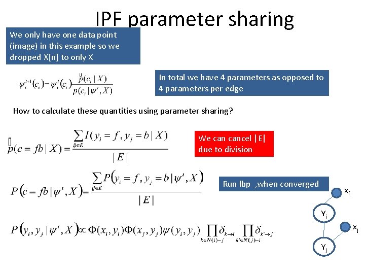
IPF parameter sharing We only have one data point (image) in this example so we dropped X[n] to only X In total we have 4 parameters as opposed to 4 parameters per edge How to calculate these quantities using parameter sharing? We cancel |E| due to division Run lbp , when converged xi Yi xj Yj