Outros mtodos n n n rvores de deciso

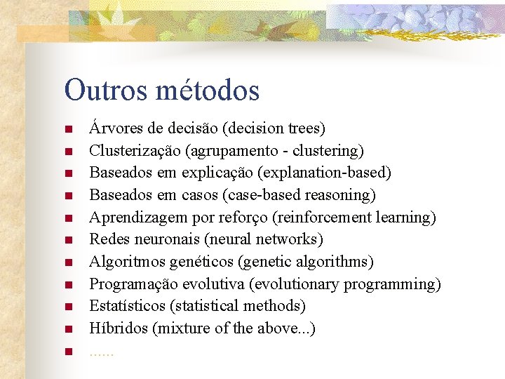
Outros métodos n n n Árvores de decisão (decision trees) Clusterização (agrupamento - clustering) Baseados em explicação (explanation-based) Baseados em casos (case-based reasoning) Aprendizagem por reforço (reinforcement learning) Redes neuronais (neural networks) Algoritmos genéticos (genetic algorithms) Programação evolutiva (evolutionary programming) Estatísticos (statistical methods) Híbridos (mixture of the above. . . ). . .

n n Programação lógica indutiva Raciocínio com incertezas

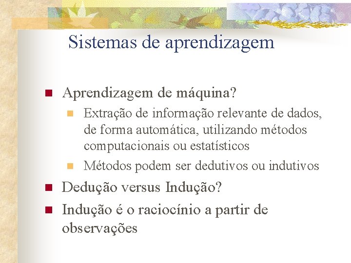
Sistemas de aprendizagem n Aprendizagem de máquina? n n Extração de informação relevante de dados, de forma automática, utilizando métodos computacionais ou estatísticos Métodos podem ser dedutivos ou indutivos Dedução versus Indução? Indução é o raciocínio a partir de observações

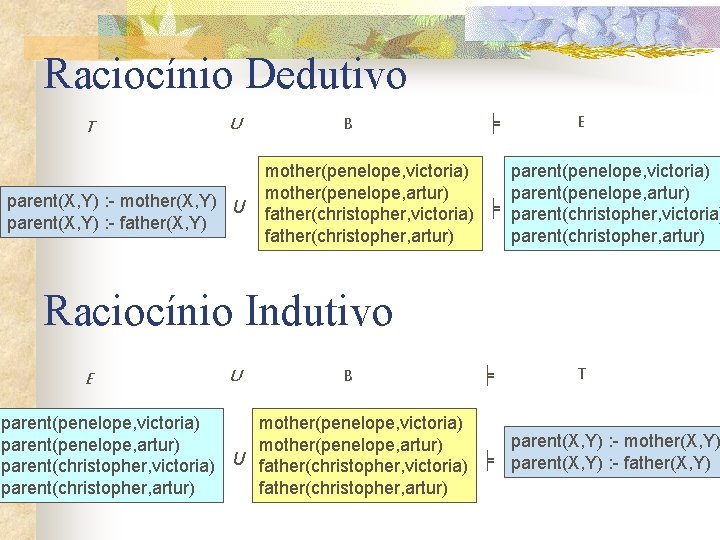
Raciocínio Dedutivo T U parent(X, Y) : - mother(X, Y) U parent(X, Y) : - father(X, Y) B ╞ E mother(penelope, victoria) parent(penelope, victoria) mother(penelope, artur) parent(penelope, artur) father(christopher, victoria) ╞ parent(christopher, victoria) father(christopher, artur) parent(christopher, artur) Raciocínio Indutivo E U B ╞ T parent(penelope, victoria) mother(penelope, victoria) parent(X, Y) : - mother(X, Y) parent(penelope, artur) mother(penelope, artur) parent(christopher, victoria) U father(christopher, victoria) ╞ parent(X, Y) : - father(X, Y) parent(christopher, artur) father(christopher, artur)

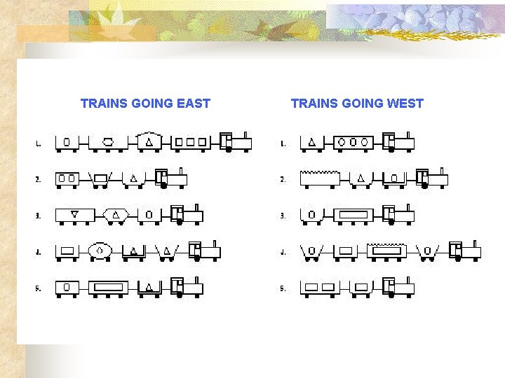
Programação Lógica Indutiva: exemplo TRAINS GOING EAST TRAINS GOING WEST

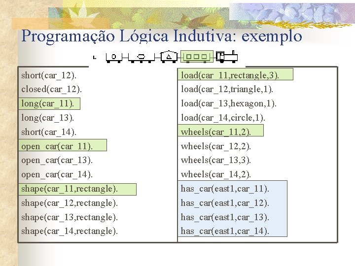
Programação Lógica Indutiva: exemplo short(car_12). closed(car_12). long(car_11). long(car_13). short(car_14). open_car(car_11). open_car(car_13). open_car(car_14). shape(car_11, rectangle). shape(car_12, rectangle). shape(car_13, rectangle). shape(car_14, rectangle). load(car_11, rectangle, 3). load(car_12, triangle, 1). load(car_13, hexagon, 1). load(car_14, circle, 1). wheels(car_11, 2). wheels(car_12, 2). wheels(car_13, 3). wheels(car_14, 2). has_car(east 1, car_11). has_car(east 1, car_12). has_car(east 1, car_13). has_car(east 1, car_14).

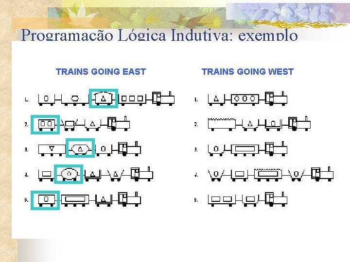
Programação Lógica Indutiva: exemplo TRAINS GOING EAST TRAINS GOING WEST

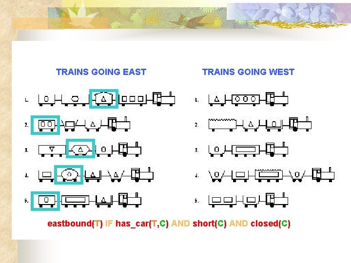
Programação Lógica Indutiva: exemplo TRAINS GOING EAST TRAINS GOING WEST eastbound(T) IF has_car(T, C) AND short(C) AND closed(C)

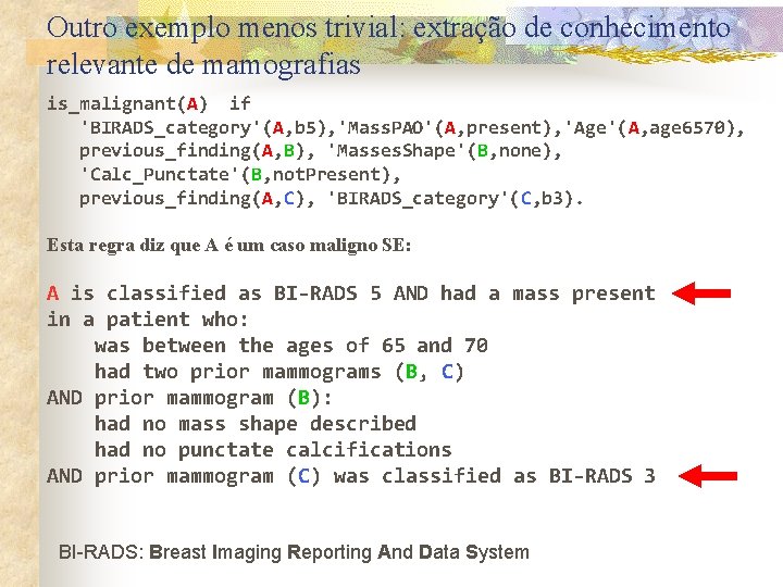
Outro exemplo menos trivial: extração de conhecimento relevante de mamografias is_malignant(A) if 'BIRADS_category'(A, b 5), 'Mass. PAO'(A, present), 'Age'(A, age 6570), previous_finding(A, B), 'Masses. Shape'(B, none), 'Calc_Punctate'(B, not. Present), previous_finding(A, C), 'BIRADS_category'(C, b 3). Esta regra diz que A é um caso maligno SE: A is classified as BI-RADS 5 AND had a mass present in a patient who: was between the ages of 65 and 70 had two prior mammograms (B, C) AND prior mammogram (B): had no mass shape described had no punctate calcifications AND prior mammogram (C) was classified as BI-RADS 3 BI-RADS: Breast Imaging Reporting And Data System

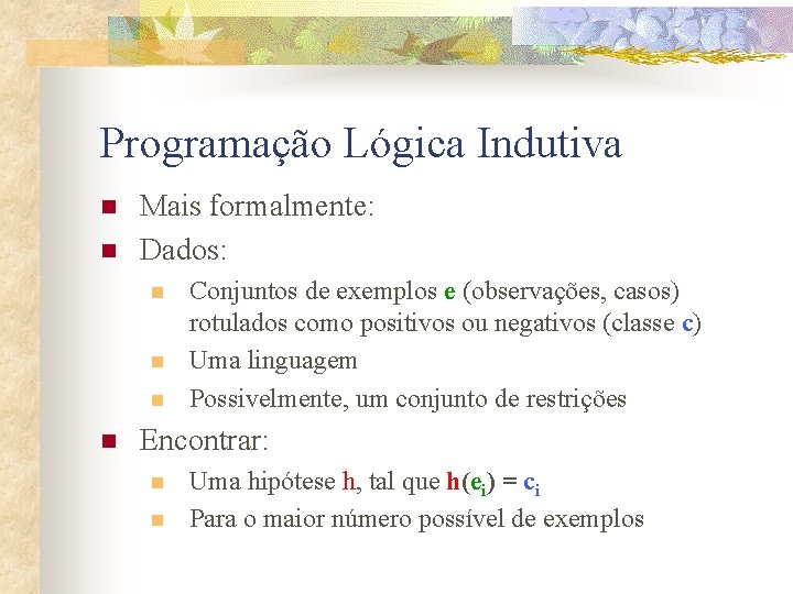
Programação Lógica Indutiva n n Mais formalmente: Dados: n n Conjuntos de exemplos e (observações, casos) rotulados como positivos ou negativos (classe c) Uma linguagem Possivelmente, um conjunto de restrições Encontrar: n n Uma hipótese h, tal que h(ei) = ci Para o maior número possível de exemplos

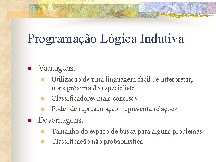
Programação Lógica Indutiva n Vantagens: n n Utilização de uma linguagem fácil de interpretar, mais próxima do especialista Classificadores mais concisos Poder de representação: representa relações Devantagens: n n Tamanho do espaço de busca para alguns problemas Classificação não probabilística

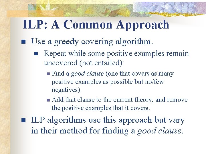
ILP: A Common Approach n Use a greedy covering algorithm. n Repeat while some positive examples remain uncovered (not entailed): n Find a good clause (one that covers as many positive examples as possible but no/few negatives). n Add that clause to the current theory, and remove the positive examples that it covers. n ILP algorithms use this approach but vary in their method for finding a good clause.

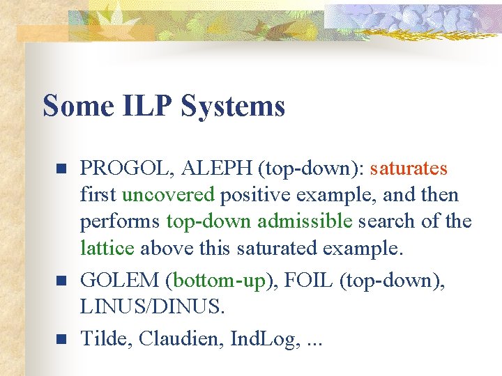
Some ILP Systems n n n PROGOL, ALEPH (top-down): saturates first uncovered positive example, and then performs top-down admissible search of the lattice above this saturated example. GOLEM (bottom-up), FOIL (top-down), LINUS/DINUS. Tilde, Claudien, Ind. Log, . . .

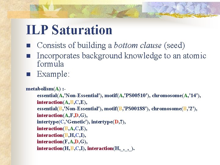
ILP Saturation n Consists of building a bottom clause (seed) Incorporates background knowledge to an atomic formula Example: metabolism(A) : essential(A, 'Non-Essential'), motif(A, 'PS 00510'), chromosome(A, '14'), interaction(A, B, C, E), essential(B, 'Non-Essential'), motif(B, 'PS 00188'), chromosome(B, '2'), interaction(A, F, D, G), intertype(C, 'Genetic'), intertype(D, ? ), interaction(B, A, C, E), interaction(B, H, C, I), interaction(F, A, D, G), interaction(H, B, C, I), interaction(H, _, _, _).

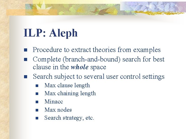
ILP: Aleph n n n Procedure to extract theories from examples Complete (branch-and-bound) search for best clause in the whole space Search subject to several user control settings n n n Max clause length Max chaining length Minacc Max nodes Search strategy, etc.

ILP: Aleph n Aleph Desenvolvido na Universidade de Oxford por Ashwin Srinivasan http: //www. comlab. ox. ac. uk/oucl/research/areas/ machlearn/Aleph/ n

ILP: Aleph Then the Rabbi said, “Golem, you have not been completely formed, but I am about to finish you now…You will do as I will tell you. ” Saying these words, Rabbi Leib finished engraving the letter Aleph. Immediately the golem began to rise.

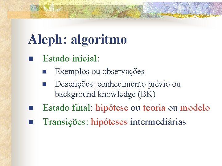
Aleph: algoritmo n Estado inicial: n n Exemplos ou observações Descrições: conhecimento prévio ou background knowledge (BK) Estado final: hipótese ou teoria ou modelo Transições: hipóteses intermediárias

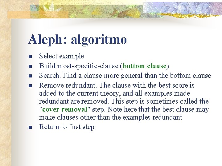
Aleph: algoritmo n n n Select example Build most-specific-clause (bottom clause) Search. Find a clause more general than the bottom clause Remove redundant. The clause with the best score is added to the current theory, and all examples made redundant are removed. This step is sometimes called the "cover removal" step. Note here that the best clause may make clauses other than the examples redundant Return to first step

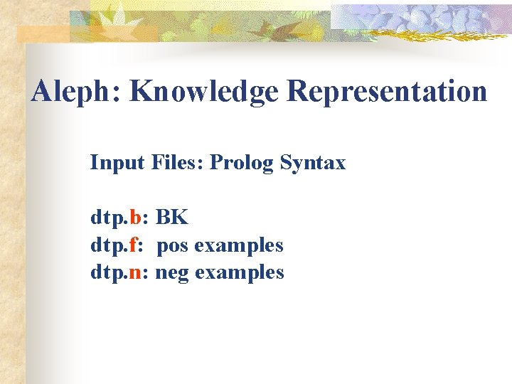
Aleph: Knowledge Representation Input Files: Prolog Syntax dtp. b: BK dtp. f: pos examples dtp. n: neg examples

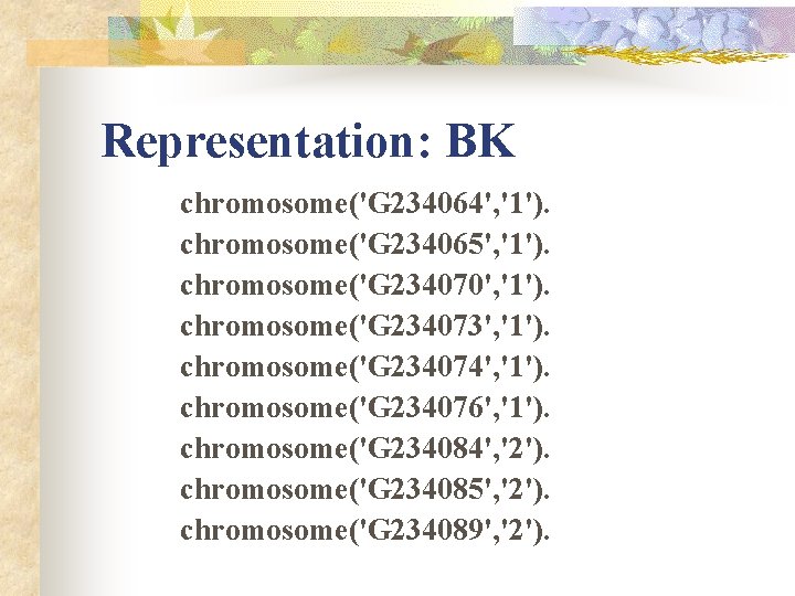
Representation: BK chromosome('G 234064', '1'). chromosome('G 234065', '1'). chromosome('G 234070', '1'). chromosome('G 234073', '1'). chromosome('G 234074', '1'). chromosome('G 234076', '1'). chromosome('G 234084', '2'). chromosome('G 234085', '2'). chromosome('G 234089', '2').

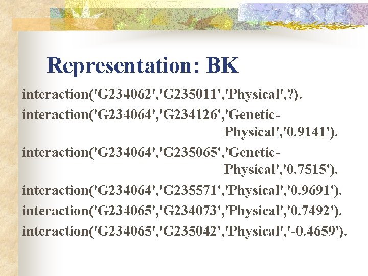
Representation: BK interaction('G 234062', 'G 235011', 'Physical', ? ). interaction('G 234064', 'G 234126', 'Genetic. Physical', '0. 9141'). interaction('G 234064', 'G 235065', 'Genetic. Physical', '0. 7515'). interaction('G 234064', 'G 235571', 'Physical', '0. 9691'). interaction('G 234065', 'G 234073', 'Physical', '0. 7492'). interaction('G 234065', 'G 235042', 'Physical', '-0. 4659').

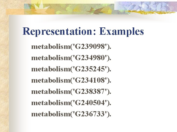
Representation: Examples metabolism('G 239098'). metabolism('G 234980'). metabolism('G 235245'). metabolism('G 234108'). metabolism('G 238387'). metabolism('G 240504'). metabolism('G 236733').

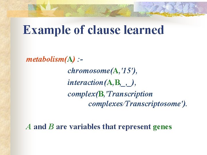
Example of clause learned metabolism(A) : chromosome(A, '15'), interaction(A, B, _, _), complex(B, 'Transcription complexes/Transcriptosome'). A and B are variables that represent genes

Aleph: algoritmo n Exemplo: trens que vão para leste e trens que vão para oeste

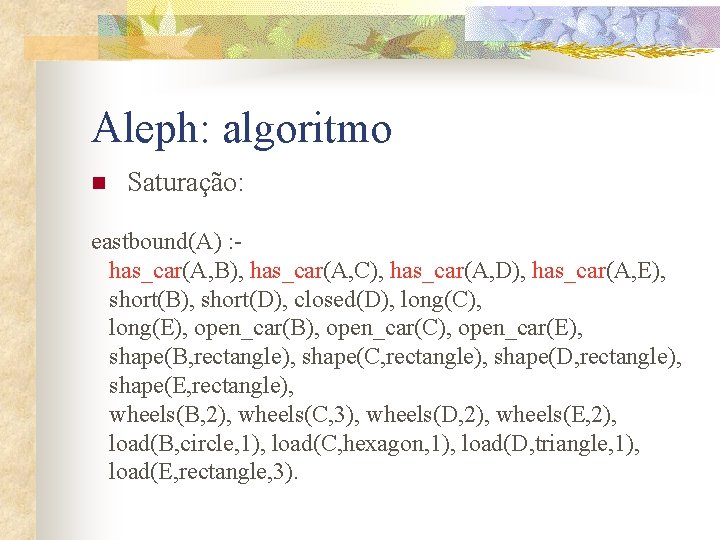
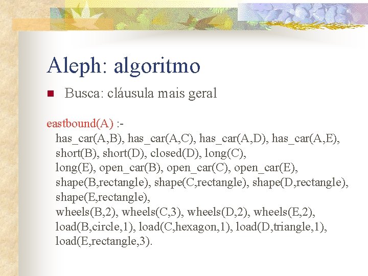
Aleph: algoritmo n Saturação: eastbound(A) : has_car(A, B), has_car(A, C), has_car(A, D), has_car(A, E), short(B), short(D), closed(D), long(C), long(E), open_car(B), open_car(C), open_car(E), shape(B, rectangle), shape(C, rectangle), shape(D, rectangle), shape(E, rectangle), wheels(B, 2), wheels(C, 3), wheels(D, 2), wheels(E, 2), load(B, circle, 1), load(C, hexagon, 1), load(D, triangle, 1), load(E, rectangle, 3).

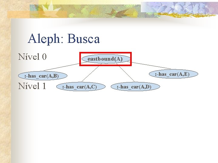
Aleph: Busca Nível 0 eastbound(A) : -has_car(A, E) : -has_car(A, B) Nível 1 : -has_car(A, C) : -has_car(A, D)

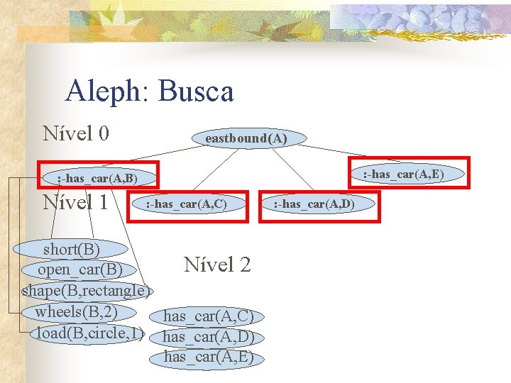
Aleph: Busca Nível 0 eastbound(A) : -has_car(A, E) : -has_car(A, B) Nível 1 : -has_car(A, C) short(B) Nível 2 open_car(B) shape(B, rectangle) wheels(B, 2) has_car(A, C) load(B, circle, 1) has_car(A, D) has_car(A, E) : -has_car(A, D)

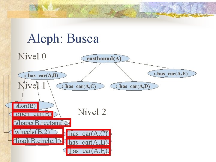
Aleph: Busca Nível 0 eastbound(A) : -has_car(A, E) : -has_car(A, B) Nível 1 short(B) : -has_car(A, C) Nível 2 open_car(B) shape(B, rectangle) wheels(B, 2) has_car(A, C) load(B, circle, 1) has_car(A, D) has_car(A, E) : -has_car(A, D)

Aleph: algoritmo n Busca: cláusula mais geral eastbound(A) : has_car(A, B), has_car(A, C), has_car(A, D), has_car(A, E), short(B), short(D), closed(D), long(C), long(E), open_car(B), open_car(C), open_car(E), shape(B, rectangle), shape(C, rectangle), shape(D, rectangle), shape(E, rectangle), wheels(B, 2), wheels(C, 3), wheels(D, 2), wheels(E, 2), load(B, circle, 1), load(C, hexagon, 1), load(D, triangle, 1), load(E, rectangle, 3).

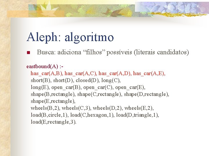
Aleph: algoritmo n Busca: adiciona “filhos” possíveis (literais candidatos) eastbound(A) : has_car(A, B), has_car(A, C), has_car(A, D), has_car(A, E), short(B), short(D), closed(D), long(C), long(E), open_car(B), open_car(C), open_car(E), shape(B, rectangle), shape(C, rectangle), shape(D, rectangle), shape(E, rectangle), wheels(B, 2), wheels(C, 3), wheels(D, 2), wheels(E, 2), load(B, circle, 1), load(C, hexagon, 1), load(D, triangle, 1), load(E, rectangle, 3).

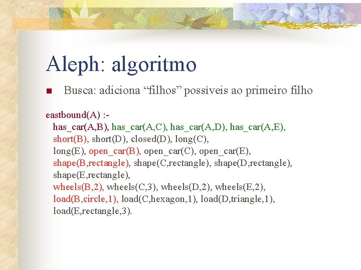
Aleph: algoritmo n Busca: adiciona “filhos” possíveis ao primeiro filho eastbound(A) : has_car(A, B), has_car(A, C), has_car(A, D), has_car(A, E), short(B), short(D), closed(D), long(C), long(E), open_car(B), open_car(C), open_car(E), shape(B, rectangle), shape(C, rectangle), shape(D, rectangle), shape(E, rectangle), wheels(B, 2), wheels(C, 3), wheels(D, 2), wheels(E, 2), load(B, circle, 1), load(C, hexagon, 1), load(D, triangle, 1), load(E, rectangle, 3).

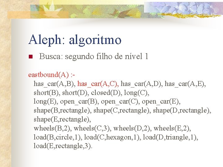
Aleph: algoritmo n Busca: segundo filho de nível 1 eastbound(A) : has_car(A, B), has_car(A, C), has_car(A, D), has_car(A, E), short(B), short(D), closed(D), long(C), long(E), open_car(B), open_car(C), open_car(E), shape(B, rectangle), shape(C, rectangle), shape(D, rectangle), shape(E, rectangle), wheels(B, 2), wheels(C, 3), wheels(D, 2), wheels(E, 2), load(B, circle, 1), load(C, hexagon, 1), load(D, triangle, 1), load(E, rectangle, 3).

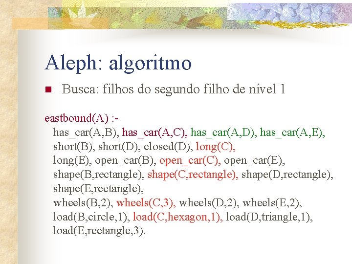
Aleph: algoritmo n Busca: filhos do segundo filho de nível 1 eastbound(A) : has_car(A, B), has_car(A, C), has_car(A, D), has_car(A, E), short(B), short(D), closed(D), long(C), long(E), open_car(B), open_car(C), open_car(E), shape(B, rectangle), shape(C, rectangle), shape(D, rectangle), shape(E, rectangle), wheels(B, 2), wheels(C, 3), wheels(D, 2), wheels(E, 2), load(B, circle, 1), load(C, hexagon, 1), load(D, triangle, 1), load(E, rectangle, 3).

Aleph: example of run aleph_trains

Aleph: how to run? n You need to have a Prolog system n n n Yap: http: //yap. sourceforge. net OU SWI: http: //www. swi-prolog. org Aleph: http: //www. comlab. ox. ac. uk/oucl/research/areas/machlearn/Aleph/ n n Files: . b, . f, . n To make things easier: everything in the same directory!

Aleph: Comandos básicos n n n read_all reduce induce

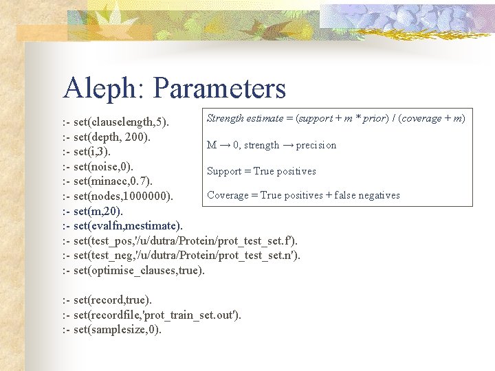
Aleph: Parameters Strength estimate = (support + m * prior) / (coverage + m) : - set(clauselength, 5). : - set(depth, 200). M → 0, strength → precision : - set(i, 3). : - set(noise, 0). Support = True positives : - set(minacc, 0. 7). Coverage = True positives + false negatives : - set(nodes, 1000000). : - set(m, 20). : - set(evalfn, mestimate). : - set(test_pos, '/u/dutra/Protein/prot_test_set. f'). : - set(test_neg, '/u/dutra/Protein/prot_test_set. n'). : - set(optimise_clauses, true). : - set(record, true). : - set(recordfile, 'prot_train_set. out'). : - set(samplesize, 0).

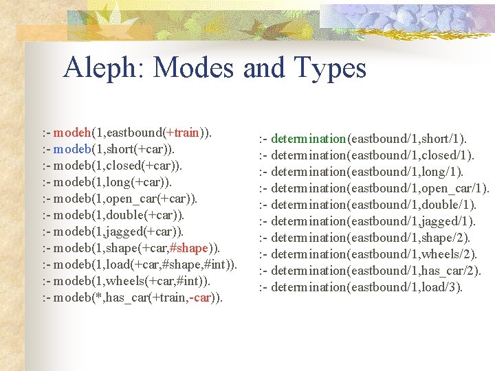
Aleph: Modes and Types : - modeh(1, eastbound(+train)). : - modeb(1, short(+car)). : - modeb(1, closed(+car)). : - modeb(1, long(+car)). : - modeb(1, open_car(+car)). : - modeb(1, double(+car)). : - modeb(1, jagged(+car)). : - modeb(1, shape(+car, #shape)). : - modeb(1, load(+car, #shape, #int)). : - modeb(1, wheels(+car, #int)). : - modeb(*, has_car(+train, -car)). : - determination(eastbound/1, short/1). : - determination(eastbound/1, closed/1). : - determination(eastbound/1, long/1). : - determination(eastbound/1, open_car/1). : - determination(eastbound/1, double/1). : - determination(eastbound/1, jagged/1). : - determination(eastbound/1, shape/2). : - determination(eastbound/1, wheels/2). : - determination(eastbound/1, has_car/2). : - determination(eastbound/1, load/3).

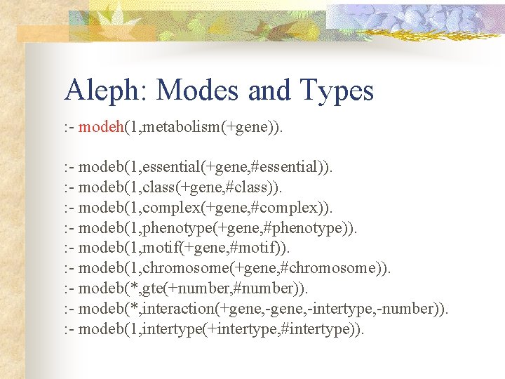
Aleph: Modes and Types : - modeh(1, metabolism(+gene)). : - modeb(1, essential(+gene, #essential)). : - modeb(1, class(+gene, #class)). : - modeb(1, complex(+gene, #complex)). : - modeb(1, phenotype(+gene, #phenotype)). : - modeb(1, motif(+gene, #motif)). : - modeb(1, chromosome(+gene, #chromosome)). : - modeb(*, gte(+number, #number)). : - modeb(*, interaction(+gene, -intertype, -number)). : - modeb(1, intertype(+intertype, #intertype)).

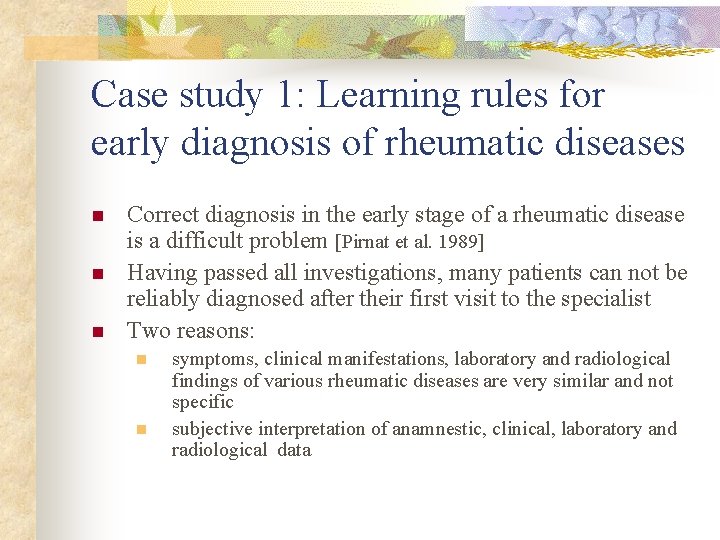
Case study 1: Learning rules for early diagnosis of rheumatic diseases n n n Correct diagnosis in the early stage of a rheumatic disease is a difficult problem [Pirnat et al. 1989] Having passed all investigations, many patients can not be reliably diagnosed after their first visit to the specialist Two reasons: n n symptoms, clinical manifestations, laboratory and radiological findings of various rheumatic diseases are very similar and not specific subjective interpretation of anamnestic, clinical, laboratory and radiological data

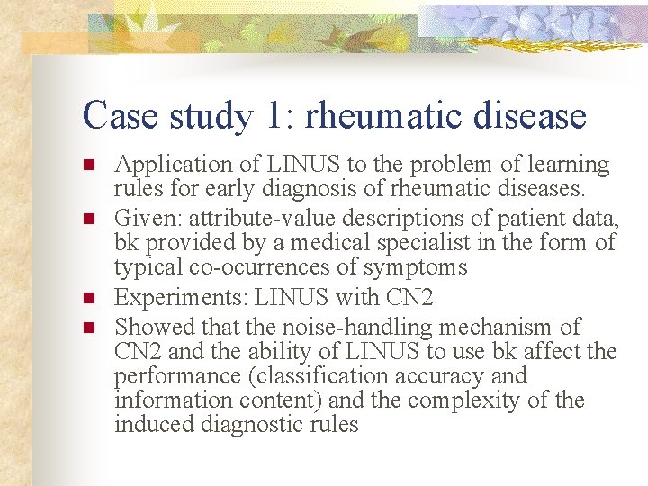
Case study 1: rheumatic disease n n Application of LINUS to the problem of learning rules for early diagnosis of rheumatic diseases. Given: attribute-value descriptions of patient data, bk provided by a medical specialist in the form of typical co-ocurrences of symptoms Experiments: LINUS with CN 2 Showed that the noise-handling mechanism of CN 2 and the ability of LINUS to use bk affect the performance (classification accuracy and information content) and the complexity of the induced diagnostic rules

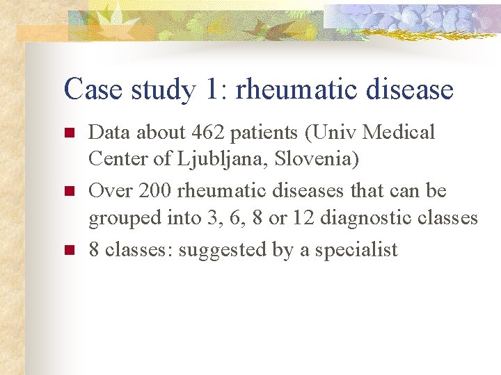
Case study 1: rheumatic disease n n n Data about 462 patients (Univ Medical Center of Ljubljana, Slovenia) Over 200 rheumatic diseases that can be grouped into 3, 6, 8 or 12 diagnostic classes 8 classes: suggested by a specialist

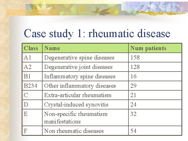
Case study 1: rheumatic disease Class A 1 A 2 B 1 B 234 C D Name Degenerative spine diseases Degenerative joint diseases Inflammatory spine diseases Other inflammatory diseases Extra-articular rheumatism Crystal-induced synovitis Num patients 158 128 16 29 21 24 E Non-specific rheumatism manifestations Non rheumatic diseases 32 F 54

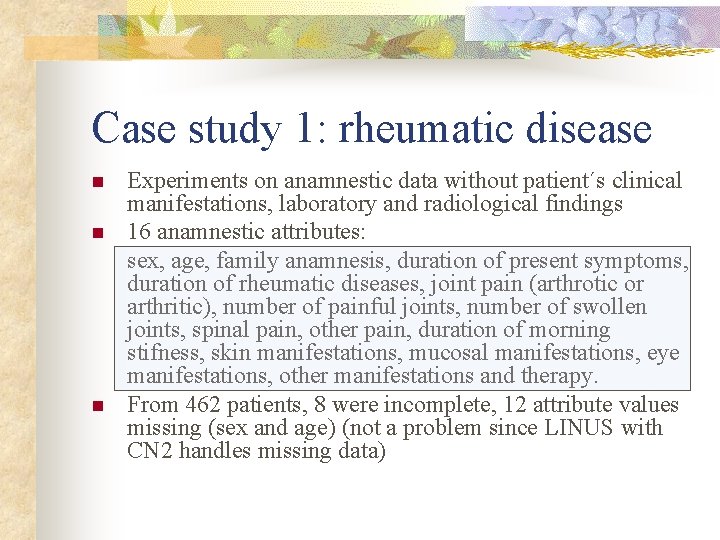
Case study 1: rheumatic disease n n n Experiments on anamnestic data without patient´s clinical manifestations, laboratory and radiological findings 16 anamnestic attributes: sex, age, family anamnesis, duration of present symptoms, duration of rheumatic diseases, joint pain (arthrotic or arthritic), number of painful joints, number of swollen joints, spinal pain, other pain, duration of morning stifness, skin manifestations, mucosal manifestations, eye manifestations, other manifestations and therapy. From 462 patients, 8 were incomplete, 12 attribute values missing (sex and age) (not a problem since LINUS with CN 2 handles missing data)

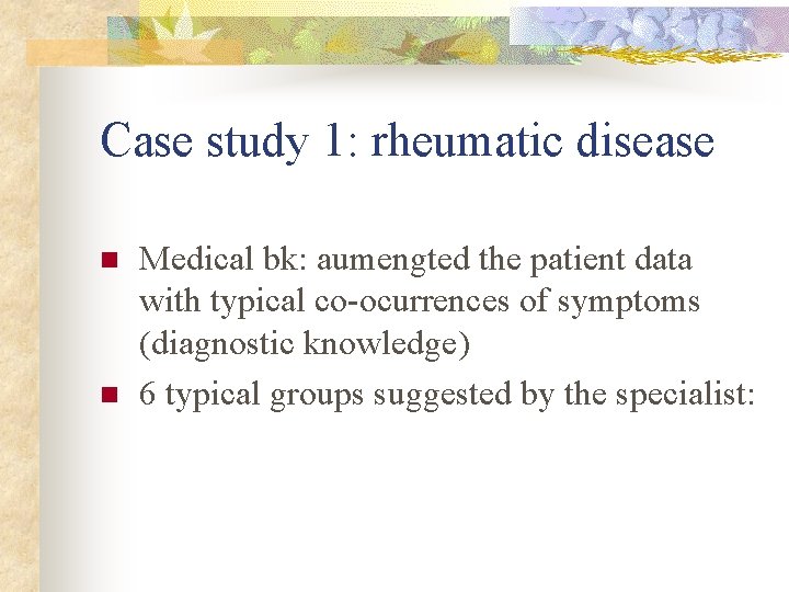
Case study 1: rheumatic disease n n Medical bk: aumengted the patient data with typical co-ocurrences of symptoms (diagnostic knowledge) 6 typical groups suggested by the specialist:

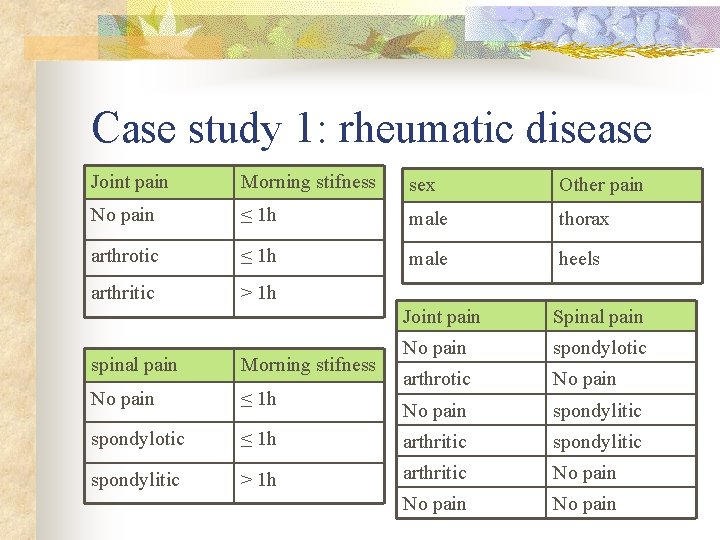
Case study 1: rheumatic disease Joint pain Morning stifness sex Other pain No pain ≤ 1 h male thorax arthrotic ≤ 1 h male heels arthritic > 1 h Joint pain Spinal pain No pain spondylotic arthrotic No pain spondylitic spinal pain Morning stifness No pain ≤ 1 h spondylotic ≤ 1 h arthritic spondylitic > 1 h arthritic No pain

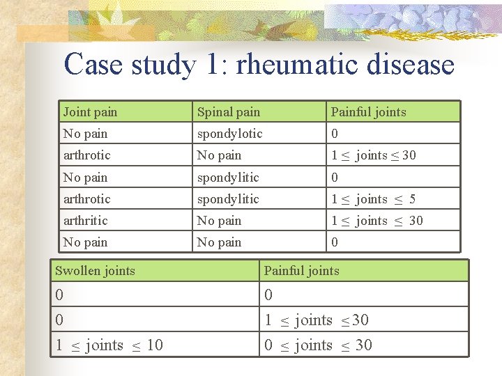
Case study 1: rheumatic disease Joint pain Spinal pain Painful joints No pain spondylotic 0 arthrotic No pain 1 ≤ joints ≤ 30 No pain spondylitic 0 arthrotic spondylitic 1 ≤ joints ≤ 5 arthritic No pain 1 ≤ joints ≤ 30 No pain 0 Swollen joints Painful joints 0 0 1 ≤ joints ≤ 10 0 1 ≤ joints ≤ 30 0 ≤ joints ≤ 30

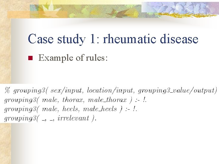
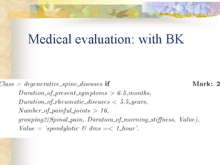
Case study 1: rheumatic disease n Example of rules:

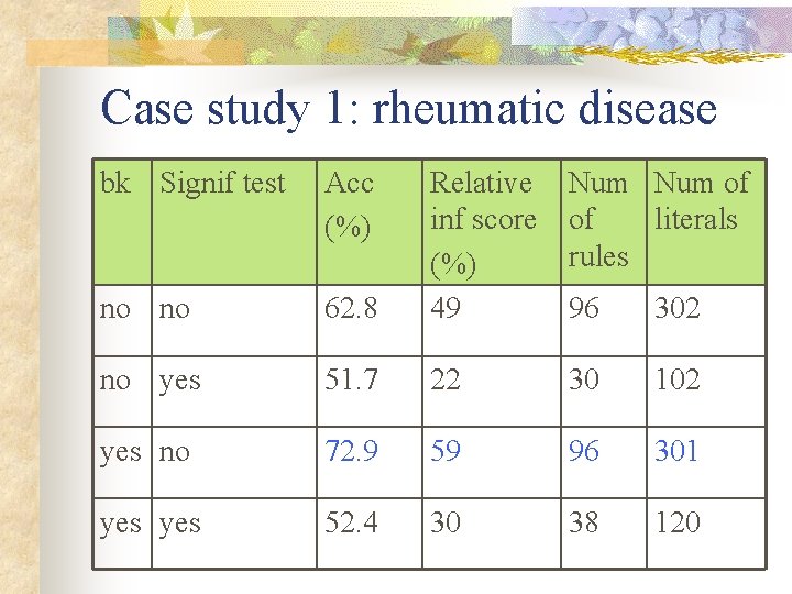
Case study 1: rheumatic disease bk Signif test Acc (%) Num of of literals rules 62. 8 Relative inf score (%) 49 no no 96 302 no yes 51. 7 22 30 102 yes no 72. 9 59 96 301 yes 52. 4 30 38 120

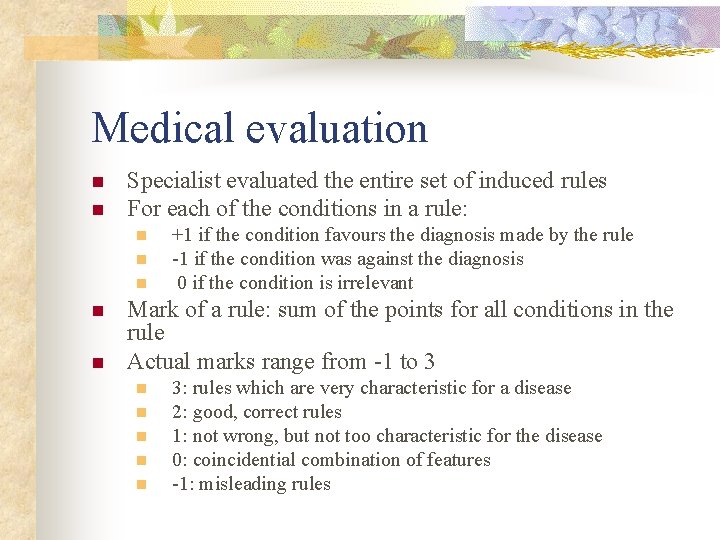
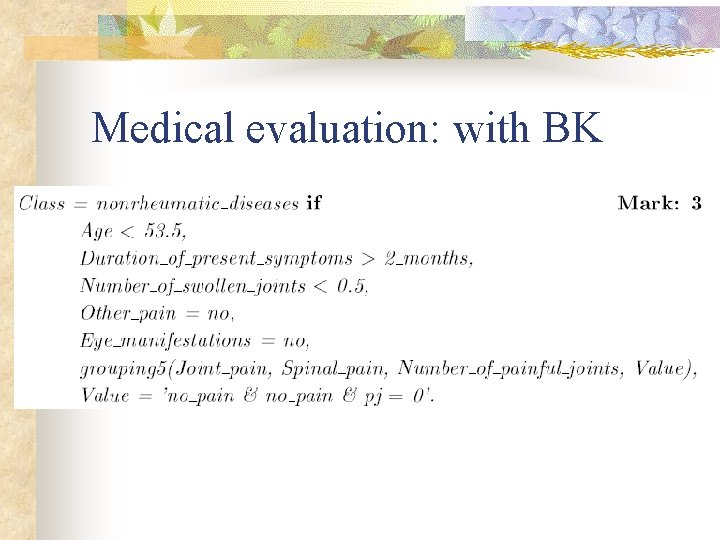
Medical evaluation n n Specialist evaluated the entire set of induced rules For each of the conditions in a rule: n n n +1 if the condition favours the diagnosis made by the rule -1 if the condition was against the diagnosis 0 if the condition is irrelevant Mark of a rule: sum of the points for all conditions in the rule Actual marks range from -1 to 3 n n n 3: rules which are very characteristic for a disease 2: good, correct rules 1: not wrong, but not too characteristic for the disease 0: coincidential combination of features -1: misleading rules

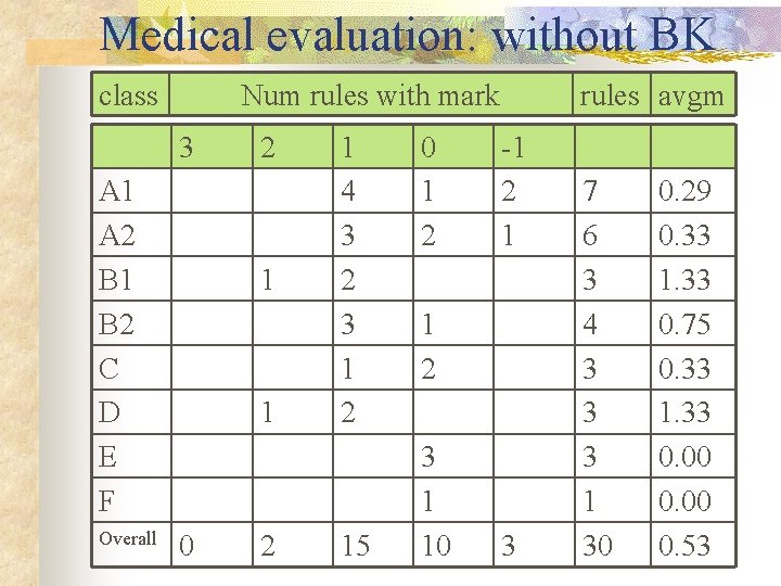
Medical evaluation: without BK class Num rules with mark 3 A 1 A 2 B 1 B 2 C D E F Overall 2 1 1 0 2 1 4 3 2 3 1 2 15 0 1 2 rules avgm -1 2 1 1 2 3 1 10 3 7 6 3 4 3 3 3 1 30 0. 29 0. 33 1. 33 0. 75 0. 33 1. 33 0. 00 0. 53

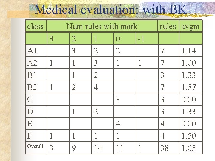
Medical evaluation: with BK class 3 A 1 A 2 B 1 B 2 C D E F Overall 1 1 1 3 Num rules with mark 2 1 0 -1 3 2 2 1 3 1 1 1 2 2 4 3 1 2 4 1 1 1 9 14 11 1 rules avgm 7 7 3 3 4 4 38 1. 14 1. 00 1. 33 1. 57 0. 00 1. 33 0. 00 1. 50 1. 05

Medical evaluation: with BK

Medical evaluation: with BK

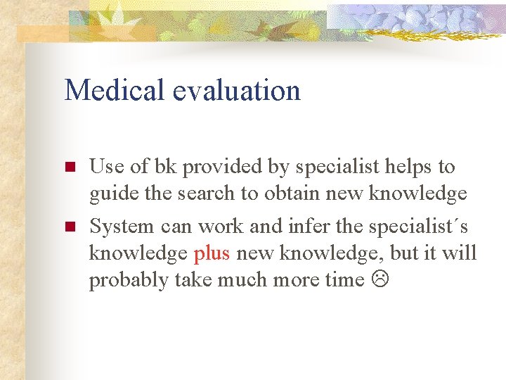
Medical evaluation n n Use of bk provided by specialist helps to guide the search to obtain new knowledge System can work and infer the specialist´s knowledge plus new knowledge, but it will probably take much more time

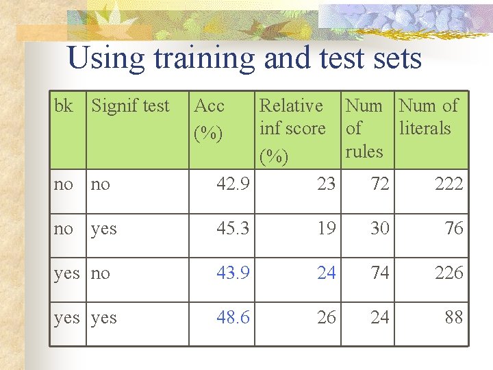
Using training ans test sets n n Four series of ten experiments 70% training, 30% test

Using training and test sets bk Signif test Acc (%) no no Relative Num of inf score of literals rules (%) 42. 9 23 72 222 no yes 45. 3 19 30 76 yes no 43. 9 24 74 226 yes 48. 6 26 24 88

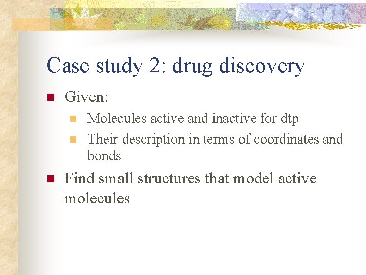
Case study 2: drug discovery n Given: n n n Molecules active and inactive for dtp Their description in terms of coordinates and bonds Find small structures that model active molecules

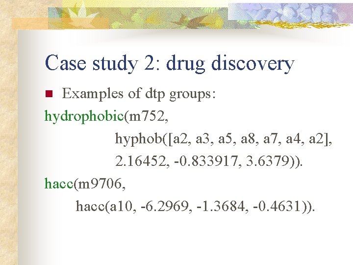
Case study 2: drug discovery Examples of dtp groups: hydrophobic(m 752, hyphob([a 2, a 3, a 5, a 8, a 7, a 4, a 2], 2. 16452, -0. 833917, 3. 6379)). hacc(m 9706, hacc(a 10, -6. 2969, -1. 3684, -0. 4631)). n

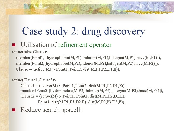
Case study 2: drug discovery n Utilisation of refinement operator refine(false, Clause): member(Point 1, [hydrophobic(M, P 1), hdonor(M, P 1), halogen(M, P 1), hacc(M, P 1)]), member(Point 2, [hydrophobic(M, P 2), hdonor(M, P 2), halogen(M, P 2), hacc(M, P 2)]), Clause = (active(M) : - Point 1, Point 2, dist(M, P 1, P 2, D 1, E)). refine(Clause 1, Clause 2): Clause 1 = (active(M) : - Point 1, Point 2, dist(M, P 1, P 2, D 1, E)), member(Point 3, [hydrophobic(M, P 3), hdonor(M, P 3), halogen(M, P 3), hacc(M, P 3)]), Clause 2 = (active(M) : - Point 1, Point 2, dist(M, P 1, P 2, D 1, E), Point 3, dist(M, P 1, P 3, D 2, E), dist(M, P 2, P 3, D 3, E)). n Reduce search space!!!

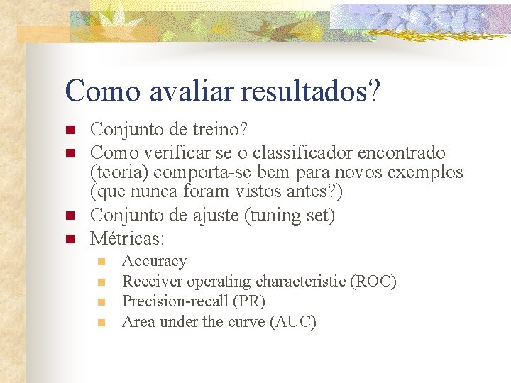
Como avaliar resultados? n n Conjunto de treino? Como verificar se o classificador encontrado (teoria) comporta-se bem para novos exemplos (que nunca foram vistos antes? ) Conjunto de ajuste (tuning set) Métricas: n n Accuracy Receiver operating characteristic (ROC) Precision-recall (PR) Area under the curve (AUC)

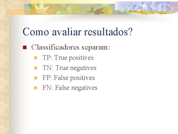
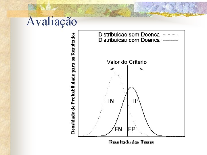
Como avaliar resultados? n Classificadores separam: n n TP: True positives TN: True negatives FP: False positives FN: False negatives

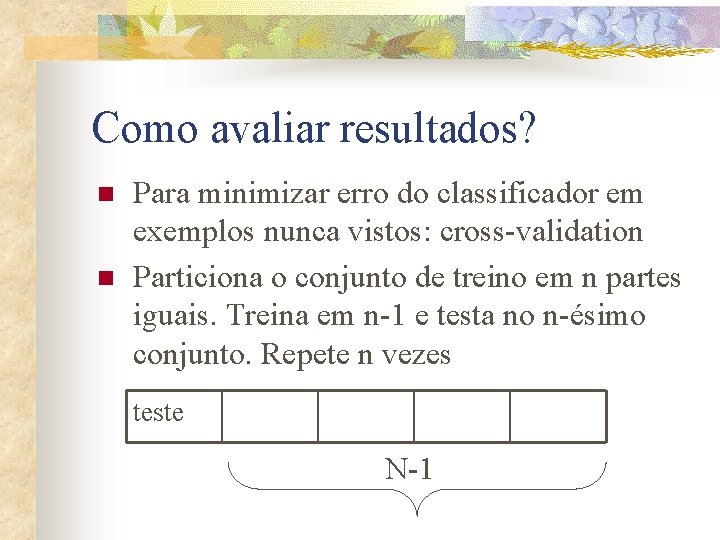
Como avaliar resultados? n n Para minimizar erro do classificador em exemplos nunca vistos: cross-validation Particiona o conjunto de treino em n partes iguais. Treina em n-1 e testa no n-ésimo conjunto. Repete n vezes teste N-1

Como avaliar resultados? n n n Leave-one-out: cross-validation onde temos n exemplos, treinamos em n-1 e deixamos 1 único exemplo para teste Problemas com cross-validation: sobreposição de exemplos em cada conjunto de treino Segundo Dietterich: 5 times 2 -fold crossvalidation should be used

Avaliação

Como avaliar resultados? n n Tuning set? Geralmente utilizado para estimar parâmetros

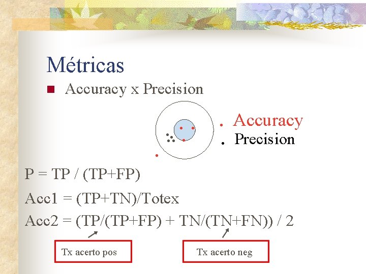
Métricas n Accuracy x Precision . Accuracy. . . . Precision. P = TP / (TP+FP) Acc 1 = (TP+TN)/Totex Acc 2 = (TP/(TP+FP) + TN/(TN+FN)) / 2 Tx acerto pos Tx acerto neg

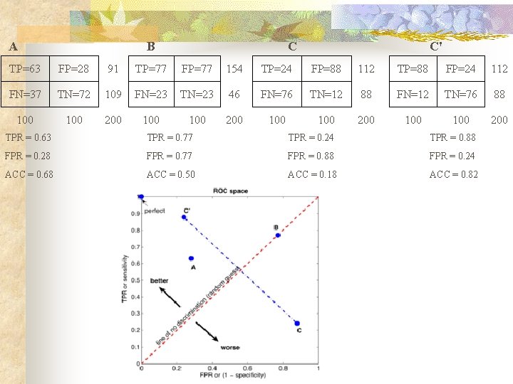
A B C C' TP=63 FP=28 91 TP=77 FP=77 154 TP=24 FP=88 112 TP=88 FP=24 112 FN=37 TN=72 109 FN=23 TN=23 46 FN=76 TN=12 88 FN=12 TN=76 88 100 100 200 TPR = 0. 63 TPR = 0. 77 TPR = 0. 24 TPR = 0. 88 FPR = 0. 28 FPR = 0. 77 FPR = 0. 88 FPR = 0. 24 ACC = 0. 68 ACC = 0. 50 ACC = 0. 18 ACC = 0. 82