Open Seminar at Tokyo Polytechnic University POD AND

Open Seminar at Tokyo Polytechnic University POD AND NEW INSIGHTS IN WIND ENGINEERING LE THAI HOA Vietnam National University, Hanoi PART 1

CONTENTS Introduction POD and its Proper Transformations in Time Domain and Frequency Domain New Insights in Wind Engineering Topic 1: POD and Pressure Fields Topic 2: POD and Wind Fields, Wind Simulation Topic 3: POD and Response Prediction Topic 4: POD and System Identification Further Perspectives and Development

BRIEF PROFILE Global COE Associate Professor Global Center of Excellence (GCOE) Program Wind Engineering Research Center (WERC) Tokyo Polytechnic University (TPU) 1583 Iiyama, Atsugi, Kanagawa, Japan, 243 -0297 Email. thle@arch. t-kougei. ac. jp On the temporary leave from Vietnam National University, Hanoi (VNU) College of Technology (COLTECH) Faculty of Engineering Mechanics 144 Xuanthuy, Caugiay, Hanoi Email. thle@vnu. edu. vn • Education • Working Experience • Research Experience • Awards

Research Experience and Interests n Wind-induced vibrations of civil structures with emphasis on aeroelastic stability analysis (Flutter Instability); Gust response prediction (Buffeting Response) of structures; Cable aerodynamics n Wind-resistant design of structures with coding and specification; wind tunnel tests n Proper Orthogonal Decomposition and its Proper Transformations with applicable for analysis, simulation, response prediction and system identification of wind effects on structures n Time – Frequency Analysis (TFA) and its Applications with applicable for analysis, simulation, response prediction and system identification of wind effects on structures n Structural Health Monitoring and Assessments

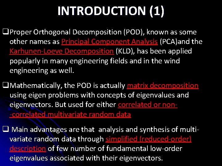
INTRODUCTION (1) q. Proper Orthogonal Decomposition (POD), known as some other names as Principal Component Analysis (PCA)and the Karhunen-Loeve Decomposition (KLD), has been applied popularly in many engineering fields and in the wind engineering as well. q. Mathematically, the POD is actually matrix decomposition using eigen problems with concepts of eigenvalues and eigenvectors. But used for either correlated or non-correlated multivariate random data q Main advantages are that analysis and synthesis of multivariate random data through simplified (reduced-order) description of few number of fundamental low-order eigenvalues associated with their eigenvectors.

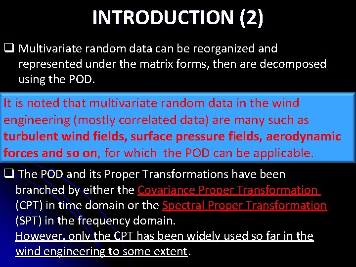
INTRODUCTION (2) q Multivariate random data can be reorganized and represented under the matrix forms, then are decomposed using the POD. It is. Normally, noted that multivariate random data in the wind q either zero-time-lag covariance matrix or cross spectral matrix of the multivariate random data such are used, engineering (mostly correlated data) are many as corresponding to the time domain and the frequency domain turbulent wind fields, surface pressure fields, aerodynamic formulations forces and so on, for which the POD can be applicable. q The POD and its Proper Transformations have been branched by either the Covariance Proper Transformation (CPT) in time domain or the Spectral Proper Transformation (SPT) in the frequency domain. However, only the CPT has been widely used so far in the wind engineering to some extent.

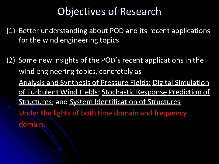
Objectives of Research (1) Better understanding about POD and its recent applications for the wind engineering topics (2) Some new insights of the POD’s recent applications in the wind engineering topics, concretely as Analysis and Synthesis of Pressure Fields; Digital Simulation of Turbulent Wind Fields; Stochastic Response Prediction of Structures; and System Identification of Structures Under the lights of both time domain and frequency domain.

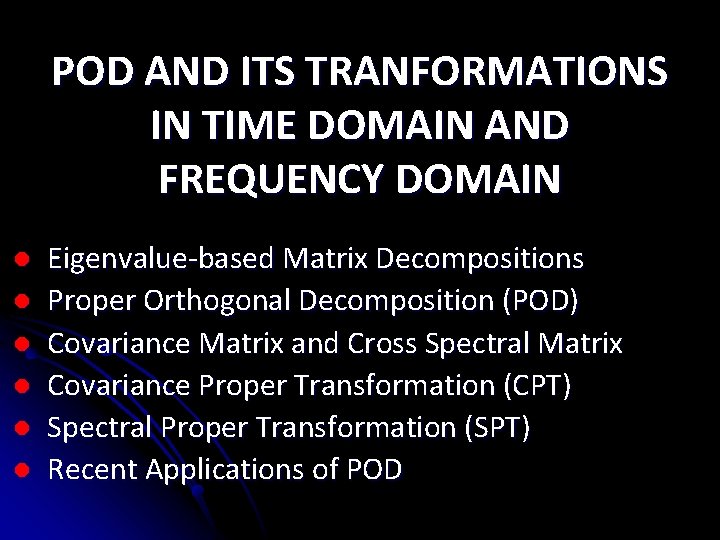
POD AND ITS TRANFORMATIONS IN TIME DOMAIN AND FREQUENCY DOMAIN l l l Eigenvalue-based Matrix Decompositions Proper Orthogonal Decomposition (POD) Covariance Matrix and Cross Spectral Matrix Covariance Proper Transformation (CPT) Spectral Proper Transformation (SPT) Recent Applications of POD

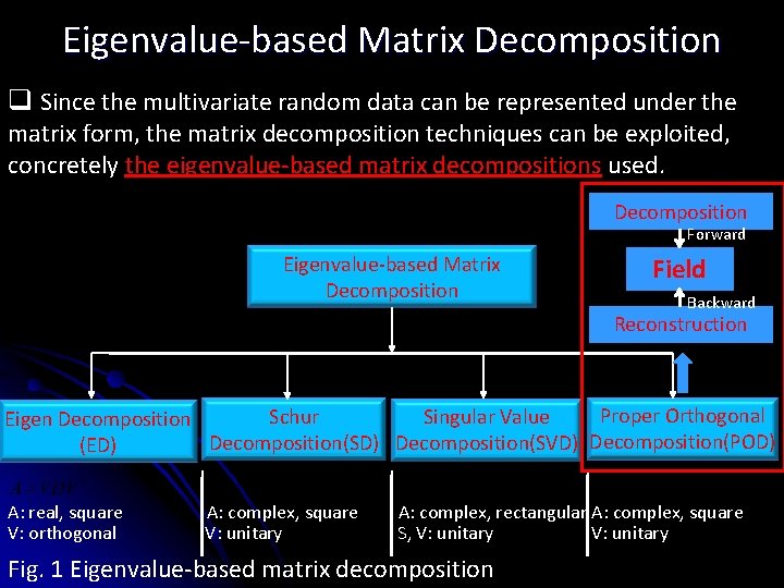
Eigenvalue-based Matrix Decomposition q Since the multivariate random data can be represented under the matrix form, the matrix decomposition techniques can be exploited, concretely the eigenvalue-based matrix decompositions used. Decomposition Forward Eigenvalue-based Matrix Decomposition Field Backward Reconstruction Proper Orthogonal Schur Singular Value Eigen Decomposition(SD) Decomposition(SVD) Decomposition(POD) (ED) A: real, square V: orthogonal A: complex, square V: unitary A: complex, rectangular A: complex, square S, V: unitary Fig. 1 Eigenvalue-based matrix decomposition

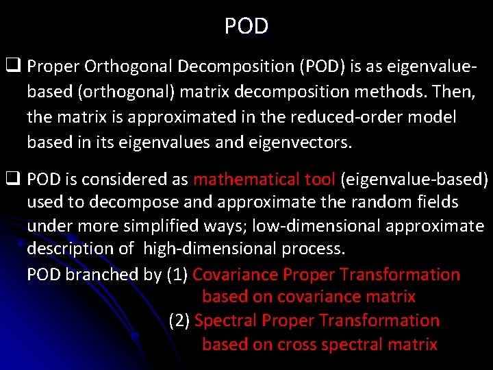
POD q Proper Orthogonal Decomposition (POD) is as eigenvaluebased (orthogonal) matrix decomposition methods. Then, the matrix is approximated in the reduced-order model based in its eigenvalues and eigenvectors. q POD is considered as mathematical tool (eigenvalue-based) used to decompose and approximate the random fields under more simplified ways; low-dimensional approximate description of high-dimensional process. POD branched by (1) Covariance Proper Transformation based on covariance matrix (2) Spectral Proper Transformation based on cross spectral matrix

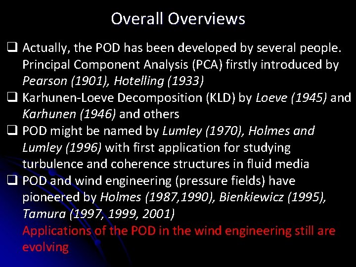
Overall Overviews q Actually, the POD has been developed by several people. Principal Component Analysis (PCA) firstly introduced by Pearson (1901), Hotelling (1933) q Karhunen-Loeve Decomposition (KLD) by Loeve (1945) and Karhunen (1946) and others q POD might be named by Lumley (1970), Holmes and Lumley (1996) with first application for studying turbulence and coherence structures in fluid media q POD and wind engineering (pressure fields) have pioneered by Holmes (1987, 1990), Bienkiewicz (1995), Tamura (1997, 1999, 2001) Applications of the POD in the wind engineering still are evolving

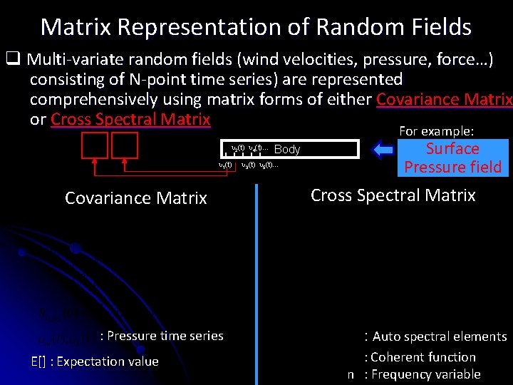
Matrix Representation of Random Fields q Multi-variate random fields (wind velocities, pressure, force…) consisting of N-point time series) are represented comprehensively using matrix forms of either Covariance Matrix or Cross Spectral Matrix For example: 2(t) 4(t)… 1(t) Covariance Matrix : Pressure time series E[] : Expectation value Body 3(t) 5(t)… Surface Pressure field Cross Spectral Matrix : Auto spectral elements : Coherent function n : Frequency variable

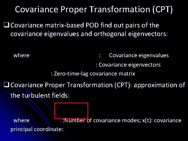
Covariance Proper Transformation (CPT) q Covariance matrix-based POD find out pairs of the covariance eigenvalues and orthogonal eigenvectors: where : Covariance eigenvalues : Covariance eigenvectors : Zero-time-lag covariance matrix q Covariance Proper Transformation (CPT): approximation of the turbulent fields: where : Number of covariance modes; x(t): covariance principal coordinate:

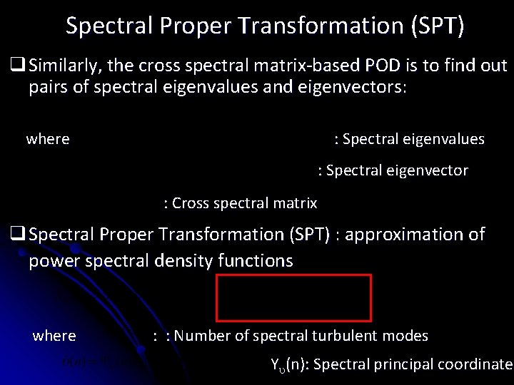
Spectral Proper Transformation (SPT) q Similarly, the cross spectral matrix-based POD is to find out pairs of spectral eigenvalues and eigenvectors: where : Spectral eigenvalues : Spectral eigenvector : Cross spectral matrix q Spectral Proper Transformation (SPT) : approximation of power spectral density functions where : : Number of spectral turbulent modes Y (n): Spectral principal coordinate

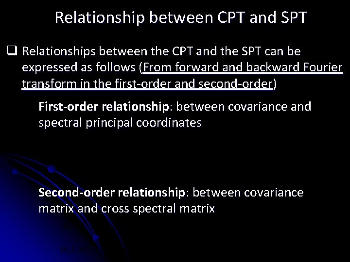
Relationship between CPT and SPT q Relationships between the CPT and the SPT can be expressed as follows (From forward and backward Fourier transform in the first-order and second-order) First-order relationship: between covariance and spectral principal coordinates Second-order relationship: between covariance matrix and cross spectral matrix

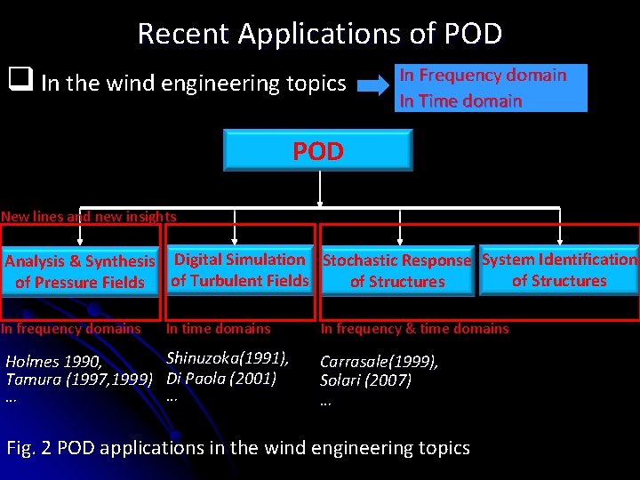
Recent Applications of POD q In the wind engineering topics In Frequency domain In Time domain POD New lines and new insights Analysis & Synthesis Digital Simulation Stochastic Response System Identification of Structures of Pressure Fields of Turbulent Fields In frequency domains Holmes 1990, Tamura (1997, 1999) … In time domains In frequency & time domains Shinuzoka(1991), Di Paola (2001) … Carrasale(1999), Solari (2007) … Fig. 2 POD applications in the wind engineering topics

NEW INSIGHTS IN WIND ENGINEERING TOPIC 1 : POD and Analysis, Synthesis and Identification of Unsteady Pressure Field l TOPIC 2 : POD and Digital Simulation of Turbulent Wind Field, Understanding Turbulent Field l TOPIC 3 : POD and Stochastic Response Prediction of Wind-excited Structures l TOPIC 4 : POD and System Identification of Wind-excited Structures l

TOPIC 1 ANALYSIS, SYNTHESIS AND IDENTIFICATION OF UNSTEADY PRESSURE FIELDS IN TIME DOMAIN AND FREQUENCY DOMAIN Introduction l Experimental set-ups l Covariance matrix-based POD analysis l Spectral matrix-based POD analysis l Identification of pressure fields and physical linkage l Results and discussions l Remarks and New Insights l

Introduction q POD has applied long stance for analyzing and identifying physical pressure fields (Holmes et al. 1988, 1997, Bienkiewicz et al. 1995, Tamura et al. 1997, 1999, 2001). q Linkage between POD modes and physical causes is usually ü looked Both covariance matrix-based POD in the time domain for to establish. and spectral matrix-based in the frequency domain Obviously, it has its advantage. POD to decompose and simplify the will be used. pressure fields. ü Linkage between the POD modes and the physical L q So far, all applications of POD for pressure fields is based phenomena on models will be investigated. on covariance matrix-based POD analysis. q. However, some literatures quoted that this physical linkages are misleading, probably fictitious in many cases due mathematical nature and sensitive constraint of POD (Armit 1967, Holme 1997, Tamura 1999).

Questionary on physical meaning “… there is no reason to suppose that spatial variation of the pressure fluctuations due to one physical cause are necessarily orthogonal with respect to that due to another cause. The mathematical constraints caused by orthogonality condition could therefore mean that in some cases, a unique physical cause cannot be associated with each eigenvector. ” Armitt, J. 1968 interpretation of physical meaning of covariance Not accurate modes might bemodes comeare from: “… the shapes of the constrained by the requirement of orthogonality, and hence any physical interpretation of these modes could be at least misleading, and (1)Number of pressure taps probably fictitious in many cases. The most useful aspect of the proper orthogonal (2)Tap arrangement or economical non-uniform) decomposition techniques (uniform is that it is an form for describing the spatial and temporal wind pressure variations on a buildings, or other bluff body, and is (3)Presence of mean pressures especially useful for relating the pressures to structural load effects. ” (4)Turbulent conditions Holmes, J. D. 1997 (5) Complexity of bluff body flow, geometry of models (6)distortion And so and on. wrong interpretation of the covariance modes due to presence of “… mean pressure data in the analyzed pressure field. ” Tamura, Y. 1997, 1999

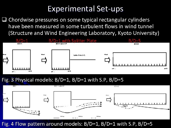
Experimental Set-ups q Chordwise pressures on some typical rectangular cylinders have been measured in some turbulent flows in wind tunnel (Structure and Wind Engineering Laboratory, Kyoto University) B/D=1 with Splitter Plate B/D=5 B/D=1 with S. P B/D=1 Wind Splitter Plate (S. P) B/D=5 Wind po 1… po 10 Fig. 3 Physical models: B/D=1, B/D=1 with S. P, B/D=5 Fig. 4 Flow pattern around models: B/D=1, B/D=1 with S. P, B/D=5 po 19

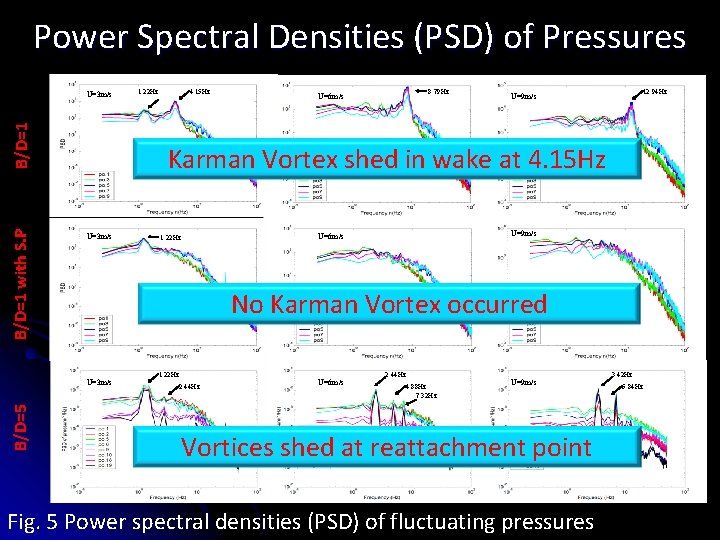
Power Spectral Densities (PSD) of Pressures B/D=1 with S. P B/D=1 U=3 m/s 4. 15 Hz 8. 79 Hz U=6 m/s 12. 94 Hz U=9 m/s Karman Vortex shed in wake at 4. 15 Hz U=3 m/s U=9 m/s U=6 m/s 1. 22 Hz No Karman Vortex occurred U=3 m/s B/D=5 1. 22 Hz 2. 44 Hz U=6 m/s 2. 44 Hz 4. 88 Hz 7. 32 Hz U=9 m/s Vortices shed at reattachment point Fig. 5 Power spectral densities (PSD) of fluctuating pressures 3. 42 Hz 6. 84 Hz

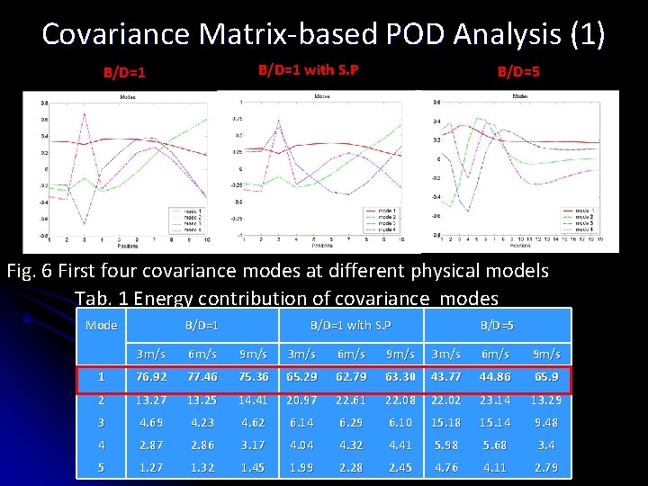
Covariance Matrix-based POD Analysis (1) B/D=1 with S. P B/D=1 B/D=5 Table 1: Energy contribution of covariance POD modes (unit: %) Fig. 6 First four covariance modes at different physical models Tab. 1 Energy contribution of covariance modes Mode B/D=1 with S. P B/D=5 3 m/s 6 m/s 9 m/s 1 76. 92 77. 46 75. 36 65. 29 62. 79 63. 30 43. 77 44. 86 65. 9 2 13. 27 13. 25 14. 41 20. 97 22. 61 22. 08 22. 02 23. 14 13. 29 3 4. 69 4. 23 4. 62 6. 14 6. 29 6. 10 15. 18 15. 14 9. 48 4 2. 87 2. 86 3. 17 4. 04 4. 32 4. 41 5. 98 5. 68 3. 4 5 1. 27 1. 32 1. 45 1. 99 2. 28 2. 45 4. 76 4. 11 2. 79

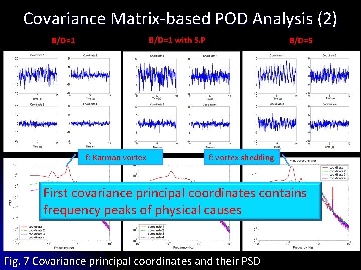
Covariance Matrix-based POD Analysis (2) B/D=1 with S. P B/D=1 f: Karman vortex 4. 15 Hz B/D=5 f: vortex shedding 1. 22 Hz First covariance principal coordinates contains frequency peaks of physical causes Fig. 7 Covariance principal coordinates and their PSD

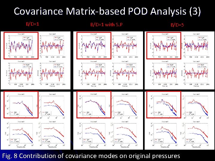
Covariance Matrix-based POD Analysis (3) B/D=1 with S. P B/D=5 Fig. 8 Contribution of covariance modes on original pressures

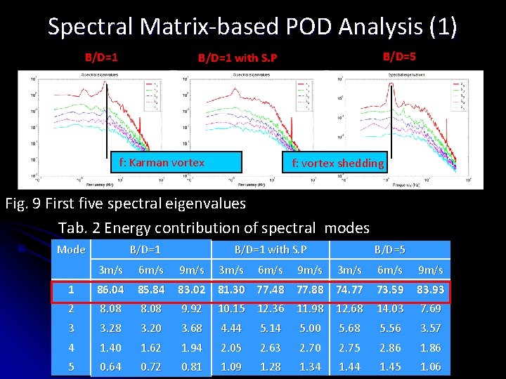
Spectral Matrix-based POD Analysis (1) B/D=1 B/D=5 B/D=1 with S. P f: Karman vortex f: vortex shedding Fig. 9 First five spectral eigenvalues Tab. 2 Energy contribution of spectral modes Mode B/D=1 with S. P 3 m/s 6 m/s 9 m/s B/D=5 3 m/s 6 m/s 9 m/s 1 86. 04 85. 84 83. 02 81. 30 77. 48 77. 88 74. 77 73. 59 83. 93 2 8. 08 9. 92 10. 15 12. 36 11. 98 12. 68 14. 03 7. 69 3 3. 28 3. 20 3. 68 4. 44 5. 14 5. 00 5. 68 5. 56 3. 57 4 1. 40 1. 62 1. 94 2. 05 2. 63 2. 70 2. 75 2. 86 1. 86 5 0. 64 0. 72 0. 81 1. 09 1. 28 1. 34 1. 45 1. 06

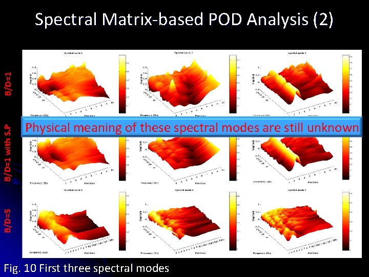
Physical meaning of these spectral modes are still unknown B/D=5 B/D=1 with S. P B/D=1 Spectral Matrix-based POD Analysis (2) Fig. 10 First three spectral modes

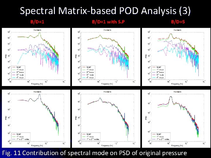
Spectral Matrix-based POD Analysis (3) B/D=1 with S. P B/D=5 Fig. 11 Contribution of spectral mode on PSD of original pressure

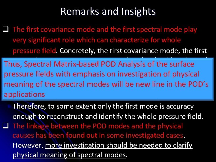
Remarks and Insights q The first covariance mode and the first spectral mode play very significant role which can characterize for whole pressure field. Concretely, the first covariance mode, the first spectral one contain certain. POD spectral peaksof ofthe hidden physical Thus, Spectral Matrix-based Analysis surface events, moreover, it contributes dominantly on the field pressure fields with emphasis on investigation of physical energy. meaning of themode spectral modes bethan newthe linecovariance in the POD’s q The spectral exhibits the will better applications mode in the synthesis (reconstruction) of the pressure field. Therefore, to some extent only the first mode is accuracy enough to reconstruct and identify the whole pressure field. q The linkage between the POD modes and the physical causes has been found out in some investigated cases. However, more investigation should be needed to clarify physical meaning of spectral modes.

TOPIC 2 DIGITAL SIMULATION OF MULTIVARIATE TURBULENT WIND FIELDS & UNDERSTANDING TURBULENT FIEDLS Introduction l Cholesky Decomposition-based Simulation l POD-based Simulation l Numerical Examples And Discussions l Investigations on Turbulent Wind Fields l Remarks and New Insights l

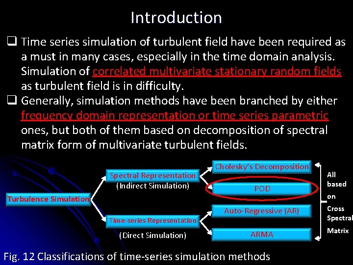
Introduction q Time series simulation of turbulent field have been required as a must in many cases, especially in the time domain analysis. Simulation of correlated multivariate stationary random fields as turbulent field is in difficulty. q Generally, simulation methods have been branched by either frequency domain representation or time series parametric ones, but both of them based on decomposition of spectral matrix form of multivariate turbulent fields. Spectral Representation (Indirect Simulation) Turbulence Simulation Time-series Representation (Direct Simulation) Cholesky’s Decomposition POD All based on Auto-Regressive (AR) Cross Spectral ARMA Matrix Fig. 12 Classifications of time-series simulation methods

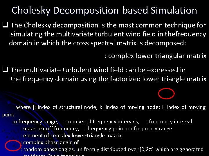
Cholesky Decomposition-based Simulation q The Cholesky decomposition is the most common technique for simulating the multivariate turbulent wind field in thefrequency domain in which the cross spectral matrix is decomposed: : complex lower triangular matrix q The multivariate turbulent wind field can be expressed in the frequency domain using the factorized lower triangle matrix where j: index of structural node; k: index of moving node; l: index of moving point in frequency range; : number of frequency intervals; : frequency interval : upper cutoff frequency; : frequency point on frequency range : element of complex lower-triangle matrix; : complex phase angle of : random phase angles, uniformly distributed over [0, 2 ] which are generated

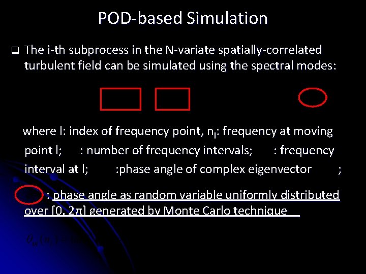
POD-based Simulation q The i-th subprocess in the N-variate spatially-correlated turbulent field can be simulated using the spectral modes: where l: index of frequency point, nl: frequency at moving point l; : number of frequency intervals; : frequency interval at l; : phase angle of complex eigenvector ; : phase angle as random variable uniformly distributed over [0, 2π] generated by Monte Carlo technique

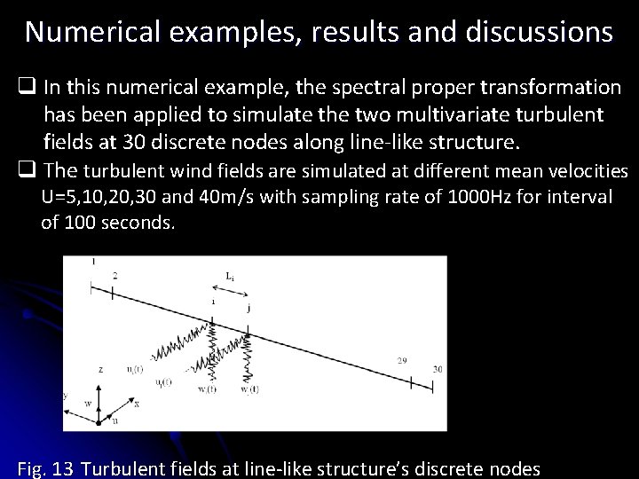
Numerical examples, results and discussions q In this numerical example, the spectral proper transformation has been applied to simulate the two multivariate turbulent fields at 30 discrete nodes along line-like structure. q The turbulent wind fields are simulated at different mean velocities U=5, 10, 20, 30 and 40 m/s with sampling rate of 1000 Hz for interval of 100 seconds. Fig. 13 Turbulent fields at line-like structure’s discrete nodes

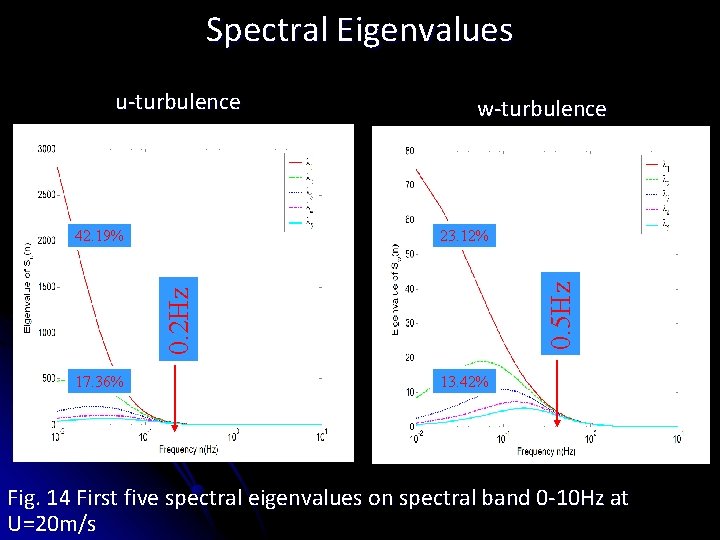
Spectral Eigenvalues u-turbulence 0. 5 Hz 23. 12% 0. 2 Hz 42. 19% w-turbulence 17. 36% 13. 42% Fig. 14 First five spectral eigenvalues on spectral band 0 -10 Hz at U=20 m/s

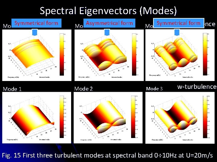
Spectral Eigenvectors (Modes) Symmetrical form Mode 1 Asymmetrical form Mode 2 Symmetrical form u-turbulence Mode 3 Mode 1 Mode 2 Mode 3 w-turbulence Fig. 15 First three turbulent modes at spectral band 0 10 Hz at U=20 m/s

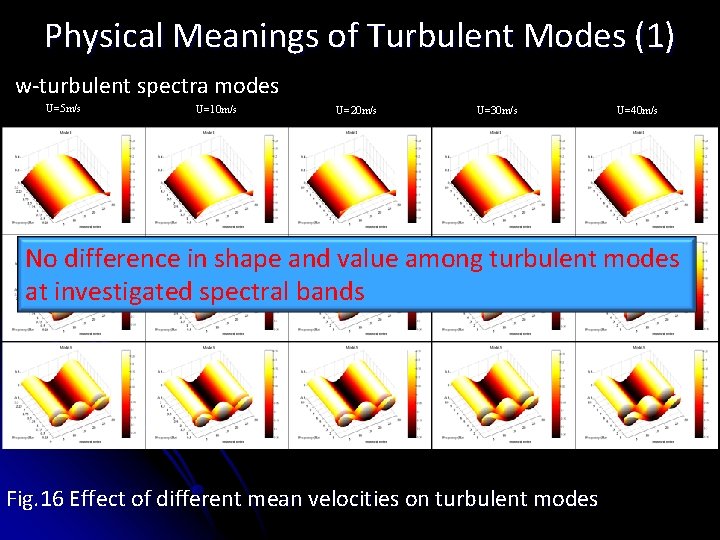
Physical Meanings of Turbulent Modes (1) w-turbulent spectra modes U=5 m/s U=10 m/s U=20 m/s U=30 m/s U=40 m/s No difference in shape and value among turbulent modes at investigated spectral bands Fig. 16 Effect of different mean velocities on turbulent modes

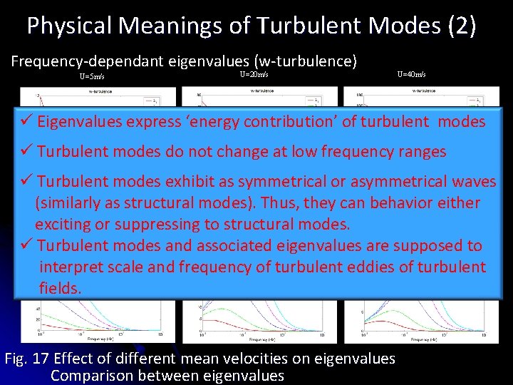
Physical Meanings of Turbulent Modes (2) Frequency-dependant eigenvalues (w-turbulence) U=5 m/s U=20 m/s U=40 m/s ü Eigenvalues express ‘energy contribution’ of turbulent modes ü Turbulent modes do not change at low frequency ranges ü Turbulent modes exhibit as symmetrical or asymmetrical waves (similarly as structural modes). Thus, they can behavior either exciting or suppressing to structural modes. ü Turbulent modes and associated eigenvalues are supposed to interpret scale and frequency of turbulent eddies of turbulent fields. Fig. 17 Effect of different mean velocities on eigenvalues Comparison between eigenvalues

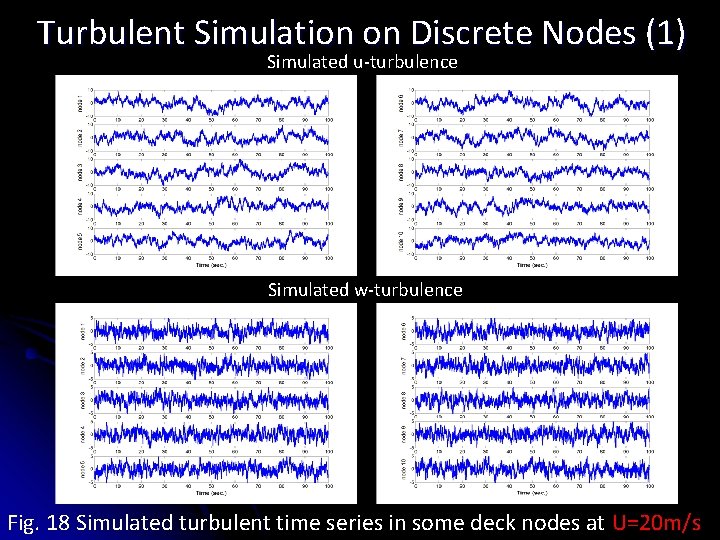
Turbulent Simulation on Discrete Nodes (1) Simulated u-turbulence Simulated w-turbulence Fig. 18 Simulated turbulent time series in some deck nodes at U=20 m/s

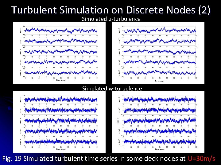
Turbulent Simulation on Discrete Nodes (2) Simulated u-turbulence Simulated w-turbulence Fig. 19 Simulated turbulent time series in some deck nodes at U=30 m/s

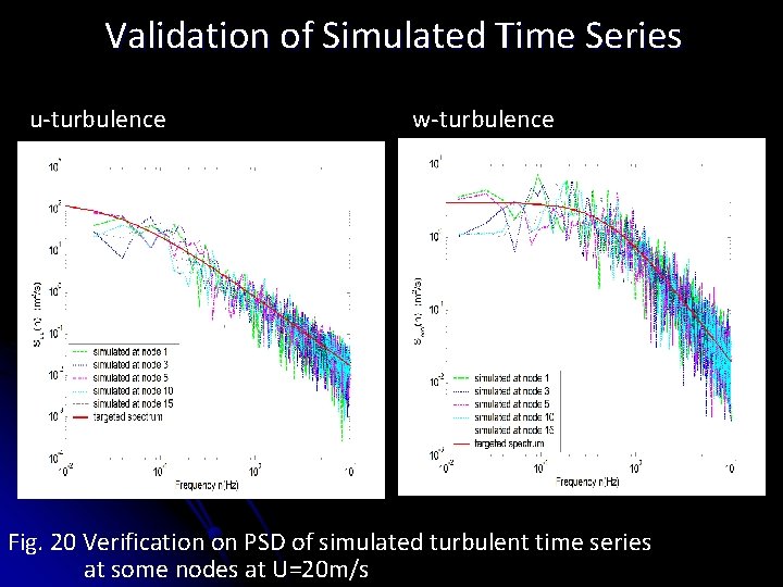
Validation of Simulated Time Series u-turbulence w-turbulence Fig. 20 Verification on PSD of simulated turbulent time series at some nodes at U=20 m/s

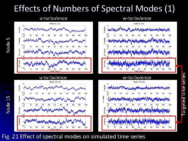
Effects of Numbers of Spectral Modes (1) w-turbulence u-turbulence w-turbulence Fig. 21 Effect of spectral modes on simulated time series Targeted time series Node 15 Node 5 u-turbulence

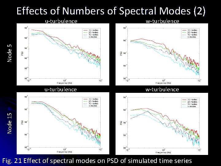
Effects of Numbers of Spectral Modes (2) u-turbulence w-turbulence Node 5 w-turbulence u-turbulence w-turbulence Node 15 w-turbulence Fig. 21 Effect of spectral modes on PSD of simulated time series

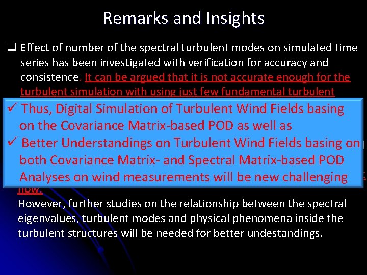
Remarks and Insights q Effect of number of the spectral turbulent modes on simulated time series has been investigated with verification for accuracy and consistence. It can be argued that it is not accurate enough for the turbulent simulation with using just few fundamental turbulent but many turbulent modes should be required ü modes, Thus, Digital Simulation of Turbulent Wind Fields basing on the meaning Covariance Matrix-based POD as well as modes q. Physical of the spectral eigenvalues and turbulent ürelating Better to Understandings Wind Fields on hidden events in on the. Turbulent ongoing turbulent flow hasbasing been tried to establish. It is expected that the. Spectral spectral eigenvalues can POD both Covariance Matrixand Matrix-based characterize scalemeasurements of the turbulent eddies of new the ongoing turbulent Analyses onforwind will be challenging flow. However, further studies on the relationship between the spectral eigenvalues, turbulent modes and physical phenomena inside the turbulent structures will be needed for better undestandings.