Name Dr Peter Tsang Room G 6505 Ext

• Name: Dr. Peter Tsang • Room: G 6505 • Ext: 7763 • Email: eewmtsan@cityu. edu. hk

• • • Introduction to Digital Signal Processing Digital Filter Design Multi-rate Signal Processing Wavelet Applications http: //www. ee. cityu. edu. hk/~csl/adsp. html

• A. N. Akansu et. al. , “Multiresolution Signal Decomposition”, Academic Press. • P. P. Vaidyanathan, “Multirate Systems and Filter Banks”, Prentice Hall. Students are strongly recommended to look for reference books in the library

Special Arrangement Class cancellation: Week 5 (6 th Oct 2007) Course Assessment: 100% Laboratory Sessions : 1 st weeks 8 2 nd weeks 10 to 13 Subject to change if necessary

Expected outcome from students: 1. 2. 3. 4. 5. Familiarize with FIR and IIR Digital Filter Design. Establish the concept of Multi-resolution Signal Decomposition. Understanding the basic mathematical framework of Wavclet Decomposition. Capable of designing and building Digital Filters, Multi-resolution and Wavelet filter banks. Applying Wavelet Decomposition in image processing.

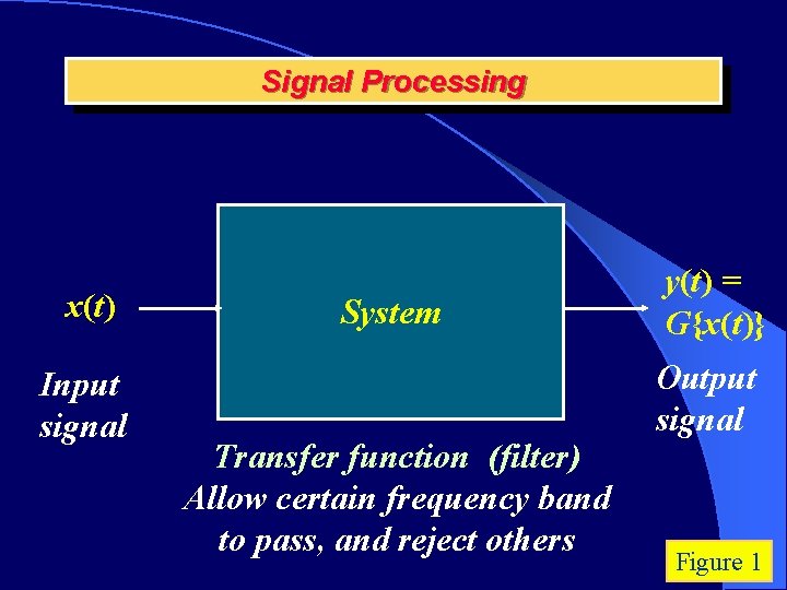
Signal Processing x(t) Input signal System Transfer function (filter) Allow certain frequency band to pass, and reject others y(t) = G{x(t)} Output signal Figure 1

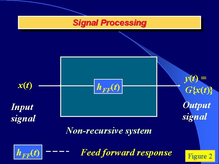
Signal Processing x(t) h. FF(t) y(t) = G{x(t)} Output signal Input signal Non-recursive system h. FF(t) Feed forward response Figure 2

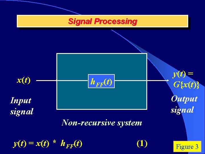
Signal Processing x(t) y(t) = G{x(t)} h. FF(t) Output signal Input signal Non-recursive system y(t) = x(t) * h. FF(t) (1) Figure 3

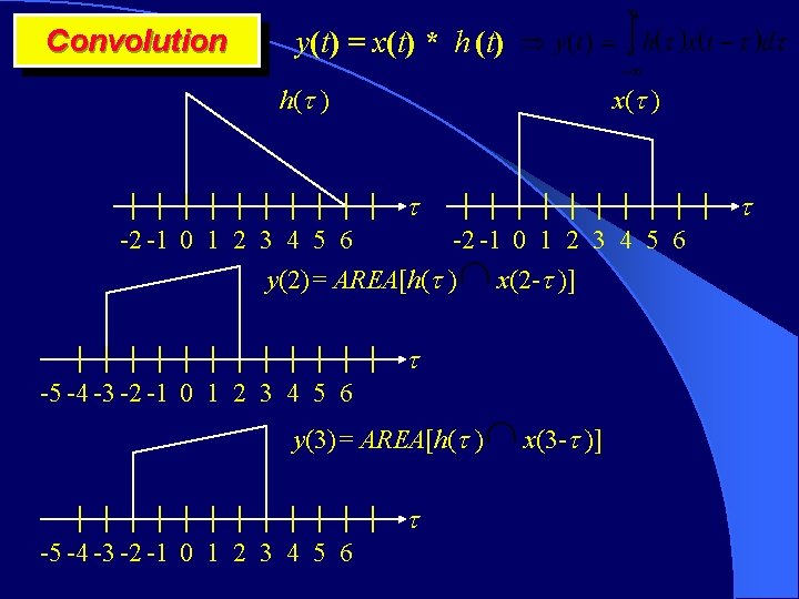
Convolution y(t) = x(t) * h (t) h( ) x( ) -2 -1 0 1 2 3 4 5 6 y(0)= AREA[h( ) -2 -1 0 1 2 3 4 5 6 x(- )] -5 -4 -3 -2 -1 0 1 2 3 4 5 6 y(1)= AREA[h( ) -5 -4 -3 -2 -1 0 1 2 3 4 5 6 x(1 - )]

Convolution y(t) = x(t) * h (t) h( ) x( ) -2 -1 0 1 2 3 4 5 6 y(2)= AREA[h( ) x(2 - )] -5 -4 -3 -2 -1 0 1 2 3 4 5 6 y(3)= AREA[h( ) -5 -4 -3 -2 -1 0 1 2 3 4 5 6 x(3 - )]

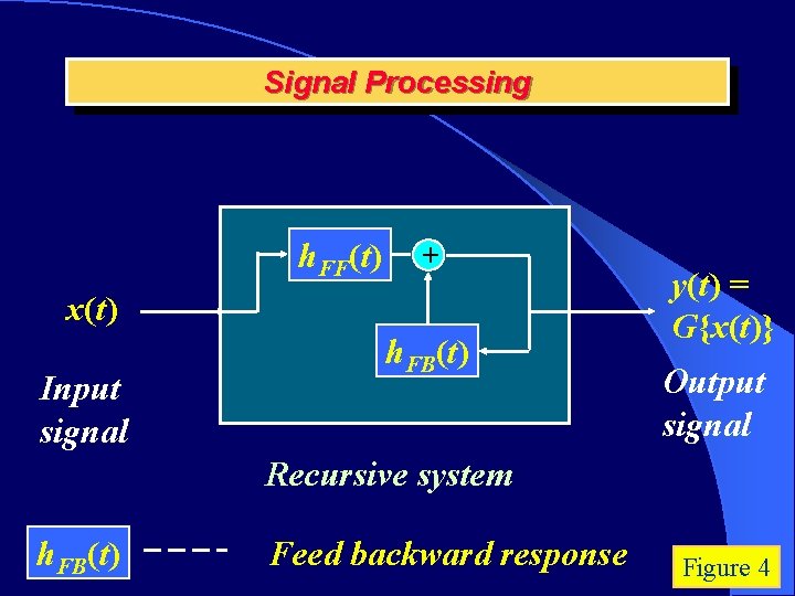
Signal Processing h. FF(t) + x(t) Input signal h. FB(t) y(t) = G{x(t)} Output signal Recursive system h. FB(t) Feed backward response Figure 4

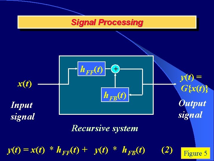
Signal Processing h. FF(t) + y(t) = G{x(t)} x(t) Input signal h. FB(t) Output signal Recursive system y(t) = x(t) * h. FF(t) + y(t) * h. FB(t) (2) Figure 5

Signal Processing Analog systems are implemented with analog circuits built up with resistors, capacitors, inductors and transistors. Both input and output signals are continuous waveforms.

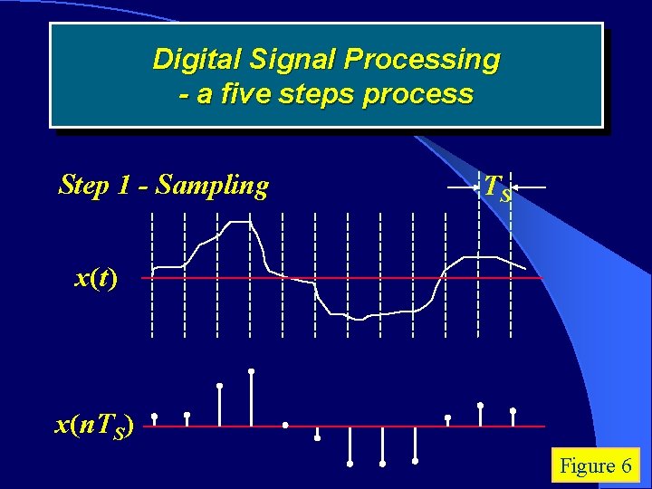
Digital Signal Processing - a five steps process Step 1 - Sampling TS x(t) x(n. TS) Figure 6

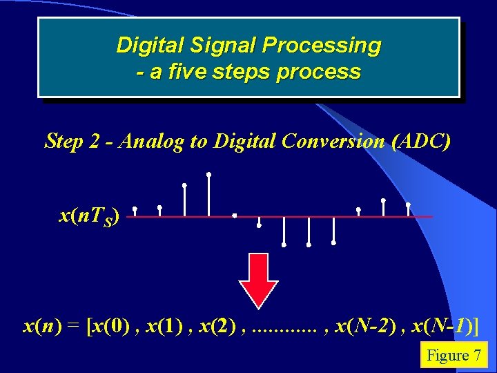
Digital Signal Processing - a five steps process Step 2 - Analog to Digital Conversion (ADC) x(n. TS) x(n) = [x(0) , x(1) , x(2) , . . . , x(N-2) , x(N-1)] Figure 7

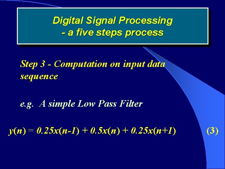
Digital Signal Processing - a five steps process Step 3 - Computation on input data sequence e. g. A simple Low Pass Filter y(n) = 0. 25 x(n-1) + 0. 5 x(n) + 0. 25 x(n+1) (3)

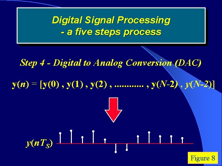
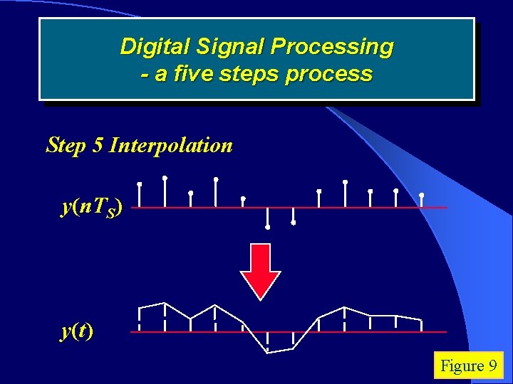
Digital Signal Processing - a five steps process Step 4 - Digital to Analog Conversion (DAC) y(n) = [y(0) , y(1) , y(2) , . . . , y(N-2)] y(n. TS) Figure 8

Digital Signal Processing - a five steps process Step 5 Interpolation y(n. TS) y(t) Figure 9

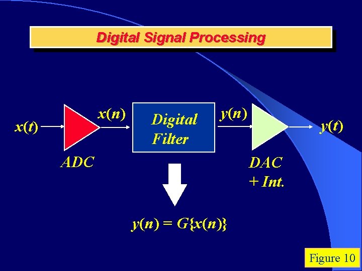
Digital Signal Processing x(n) x(t) Digital Filter y(n) ADC y(t) DAC + Int. y(n) = G{x(n)} Figure 10

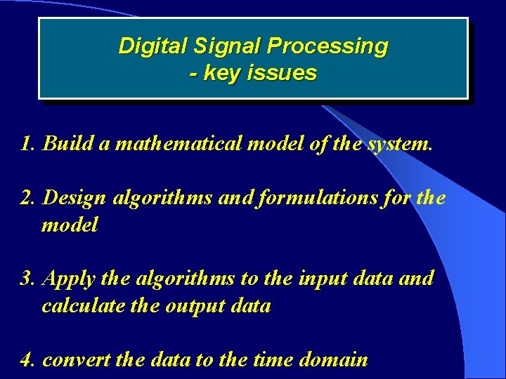
Digital Signal Processing - key issues 1. Build a mathematical model of the system. 2. Design algorithms and formulations for the model 3. Apply the algorithms to the input data and calculate the output data 4. convert the data to the time domain

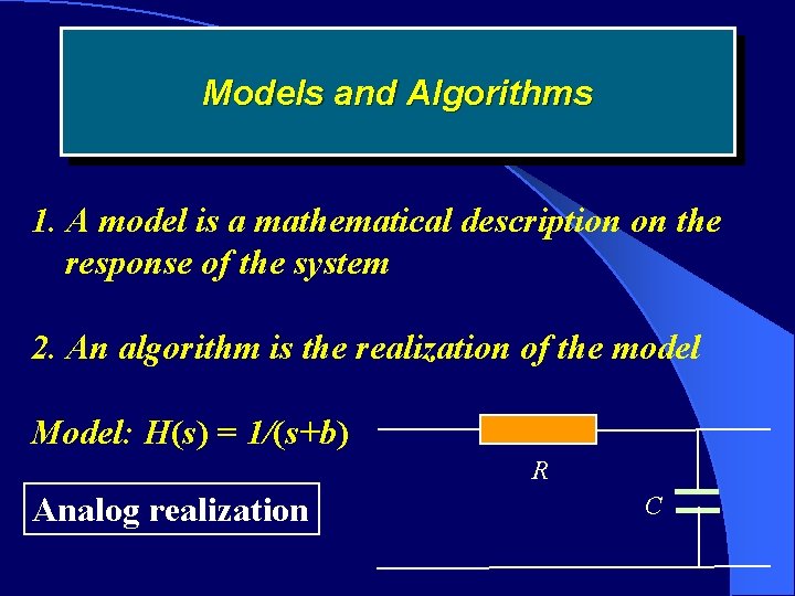
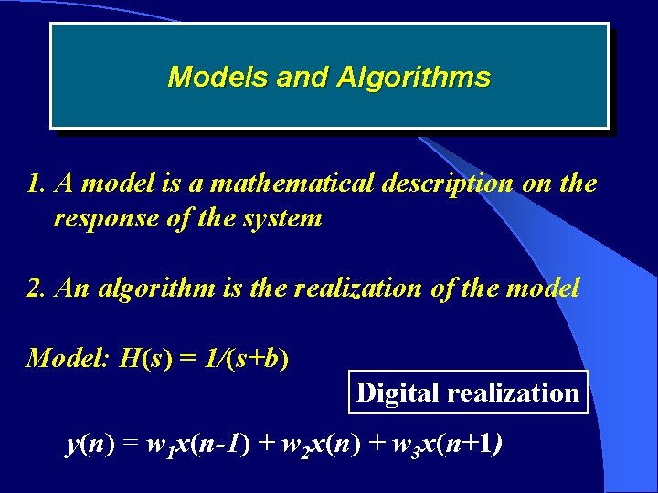
Models and Algorithms 1. A model is a mathematical description on the response of the system 2. An algorithm is the realization of the model Model: H(s) = 1/(s+b) R Analog realization C

Models and Algorithms 1. A model is a mathematical description on the response of the system 2. An algorithm is the realization of the model Model: H(s) = 1/(s+b) Digital realization y(n) = w 1 x(n-1) + w 2 x(n) + w 3 x(n+1)

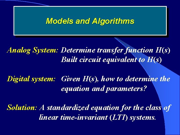
Models and Algorithms Analog System: Determine transfer function H(s) Built circuit equivalent to H(s) Digital system: Given H(s), how to determine the equation and parameters? Solution: A standardized equation for the class of linear time-invariant (LTI) systems.

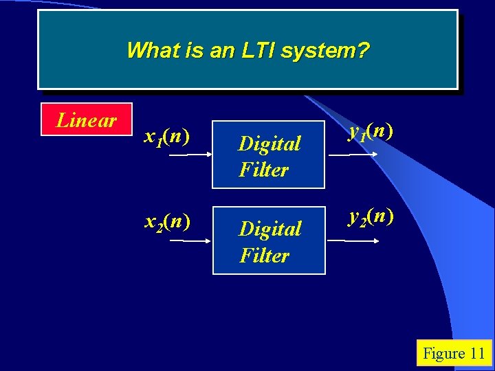
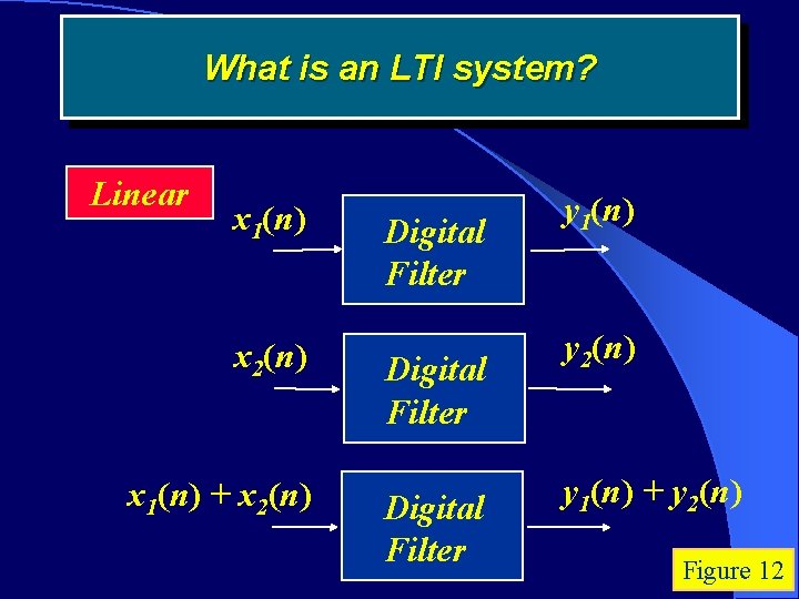
What is an LTI system? Linear x 1(n) x 2(n) Digital Filter y 1(n) y 2(n) Figure 11

What is an LTI system? Linear x 1(n) Digital Filter x 2(n) Digital Filter x 1(n) + x 2(n) Digital Filter y 1(n) y 2(n) y 1(n) + y 2(n) Figure 12

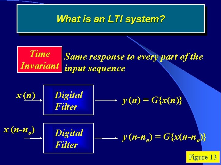
What is an LTI system? Time Same response to every part of the Invariant input sequence x (n) Digital Filter y (n) = G{x(n)} x (n-no) Digital Filter y (n-no) = G{x(n-no)} Figure 13

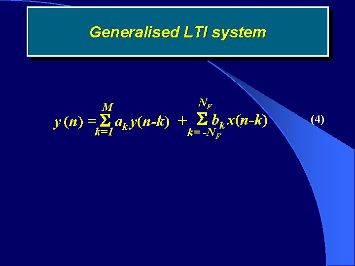
Generalised LTI system M NF k=1 k= -NF y (n) = ak y(n-k) + bk x(n-k) (4)

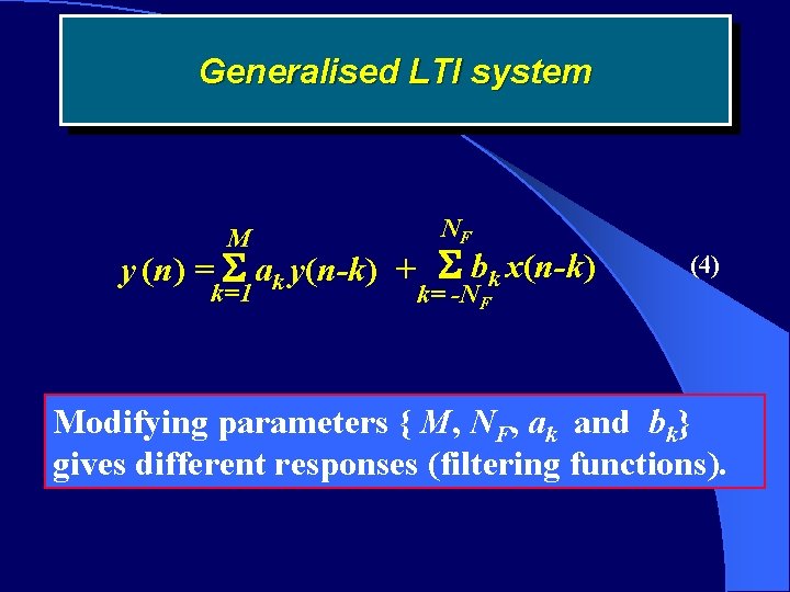
Generalised LTI system M NF k=1 k= -NF y (n) = ak y(n-k) + bk x(n-k) (4) Modifying parameters { M, NF, ak and bk} gives different responses (filtering functions).

Summary Designing analog systems • Identify the desire filter response (e. g. HP, LP, etc. )

Summary Designing analog systems • Identify the desire filter response (e. g. HP, LP, etc. ) • Determine the mathematical representation of the response H(s)

Summary Designing analog systems • Identify the desire filter response (e. g. HP, LP, etc. ) • Determine the mathematical representation of the response H(s) • Implement the filter circuit with RLC transistors and FETs

Summary Designing digital systems • Digitize the input analog signal into a sequence of data x(n) = [x(0), x(1), x(2), . . . . x(N-1)]

Summary Designing digital systems • Digitize the input analog signal into a sequence of data x(n) = [x(0), x(1), x(2), . . . . x(N-1)] • Identify the desire digital filter response (e. g. HP, LP, etc. )

Summary Designing digital systems • Digitize the input analog signal into a sequence of data x(n) = [x(0), x(1), x(2), . . . . x(N-1)] • Identify the desire digital filter response (e. g. HP, LP, etc. ) • Determine the mathematical representation of the digital response G(n)

Summary Designing digital systems • Digitize the input analog signal into a sequence of data x(n) = [x(0), x(1), x(2), . . . . x(N-1)] • Identify the desire digital filter response (e. g. HP, LP, etc. ) • Determine the mathematical representation of the digital response G(n) • Implement the digital filter with the Generalised LTI architecture

It sounds simple, but something does not fit in What is it?

It sounds simple, but something does not fit in What is it? The sequence of data x(n) = [x(0), x(1), x(2), . . . . x(N-1)] seems to be unrelated to time and frequency.

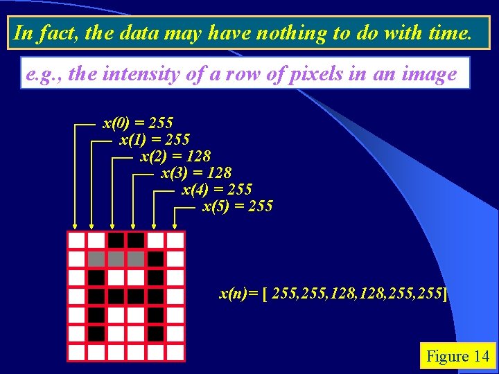
In fact, the data may have nothing to do with time. e. g. , the intensity of a row of pixels in an image x(0) = 255 x(1) = 255 x(2) = 128 x(3) = 128 x(4) = 255 x(5) = 255 x(n)= [ 255, 128, 255, 255] Figure 14

So what is meant by frequency in the digital domain?

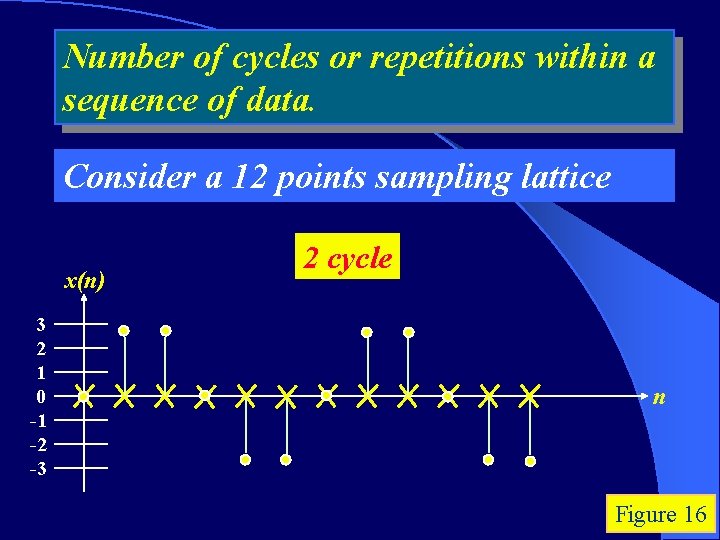
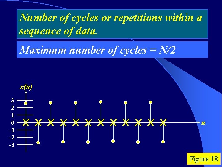
So what is meant by frequency in the digital domain? Number of cycles or repetitions within a sequence of data

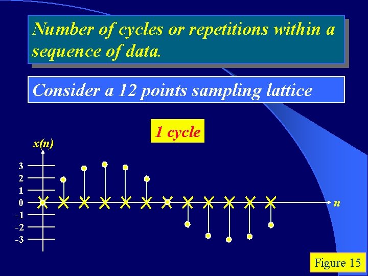
Number of cycles or repetitions within a sequence of data. Consider a 12 points sampling lattice x(n) 3 2 1 0 -1 -2 -3 1 cycle n Figure 15

Number of cycles or repetitions within a sequence of data. Consider a 12 points sampling lattice x(n) 3 2 1 0 -1 -2 -3 2 cycle n Figure 16

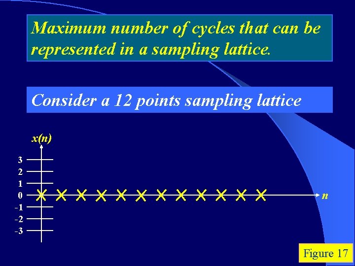
Maximum number of cycles that can be represented in a sampling lattice. Consider a 12 points sampling lattice x(n) 3 2 1 0 -1 -2 -3 n Figure 17

Number of cycles or repetitions within a sequence of data. Maximum number of cycles = N/2 x(n) 3 2 1 0 -1 -2 -3 n Figure 18

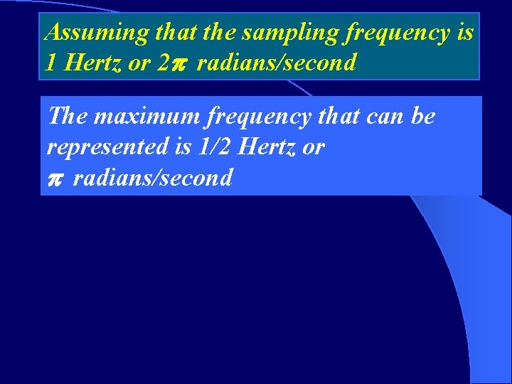
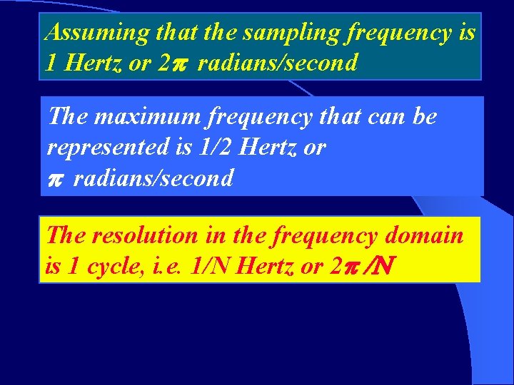
Assuming that the sampling frequency is 1 Hertz or 2 radians/second The maximum frequency that can be represented is 1/2 Hertz or radians/second

Assuming that the sampling frequency is 1 Hertz or 2 radians/second The maximum frequency that can be represented is 1/2 Hertz or radians/second The resolution in the frequency domain is 1 cycle, i. e. 1/N Hertz or 2

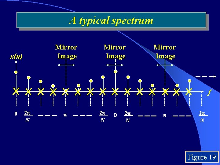
A typical spectrum Mirror Image x(n) Mirror Image f 0 2 N 2 N Figure 19

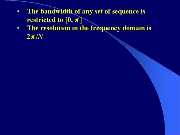
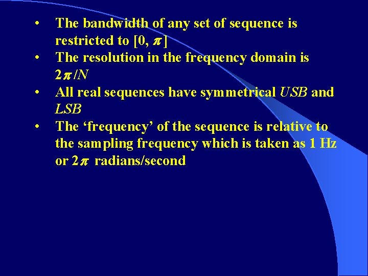
• The bandwidth of any set of sequence is restricted to [0, ]

• • The bandwidth of any set of sequence is restricted to [0, ] The resolution in the frequency domain is 2 /N

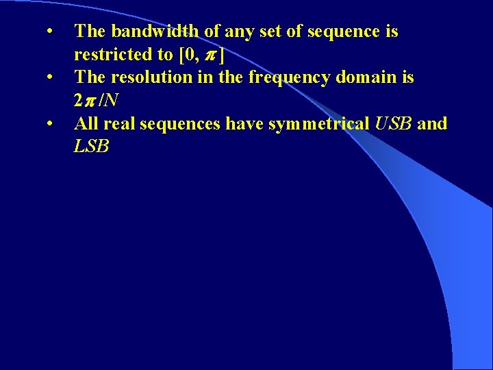
• • • The bandwidth of any set of sequence is restricted to [0, ] The resolution in the frequency domain is 2 /N All real sequences have symmetrical USB and LSB

• • The bandwidth of any set of sequence is restricted to [0, ] The resolution in the frequency domain is 2 /N All real sequences have symmetrical USB and LSB The ‘frequency’ of the sequence is relative to the sampling frequency which is taken as 1 Hz or 2 radians/second

• • The bandwidth of any set of sequence is restricted to [0, ] The resolution in the frequency domain is 2 /N All real sequences have symmetrical USB and LSB The ‘frequency’ of the sequence is relative to the sampling frequency which is taken as 1 Hz or 2 radians/second

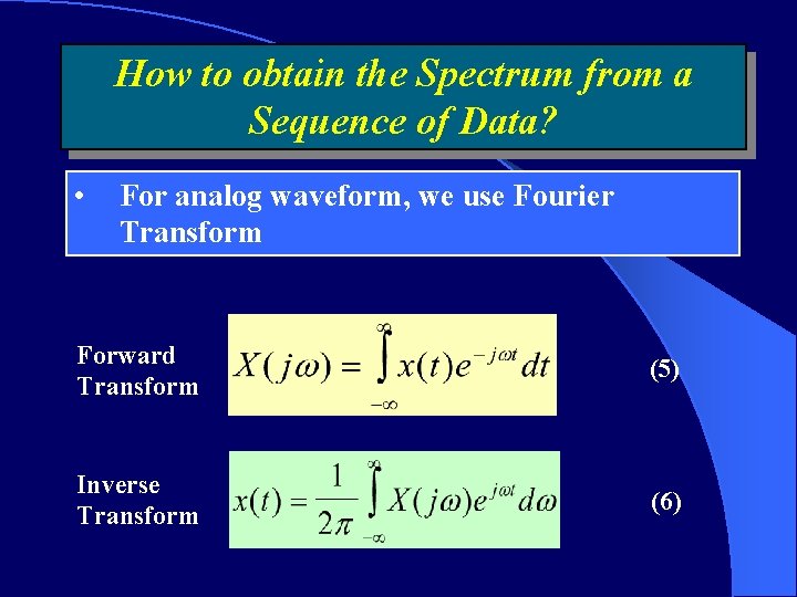
How to obtain the Spectrum from a Sequence of Data? • For analog waveform, we use Fourier Transform Forward Transform (5) Inverse Transform (6)

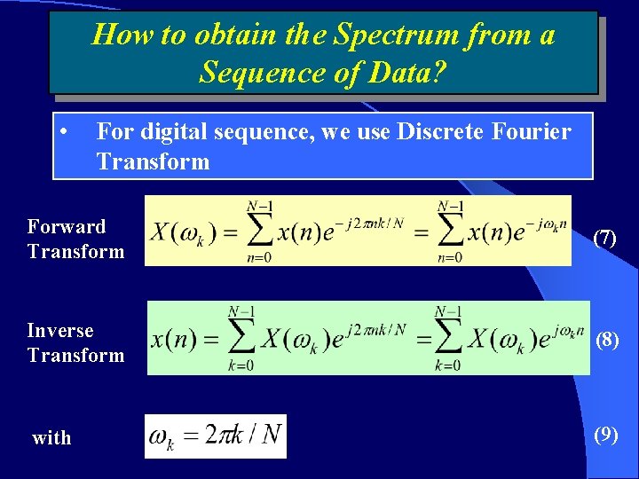
How to obtain the Spectrum from a Sequence of Data? • For digital sequence, we use Discrete Fourier Transform Forward Transform (7) Inverse Transform (8) with (9)

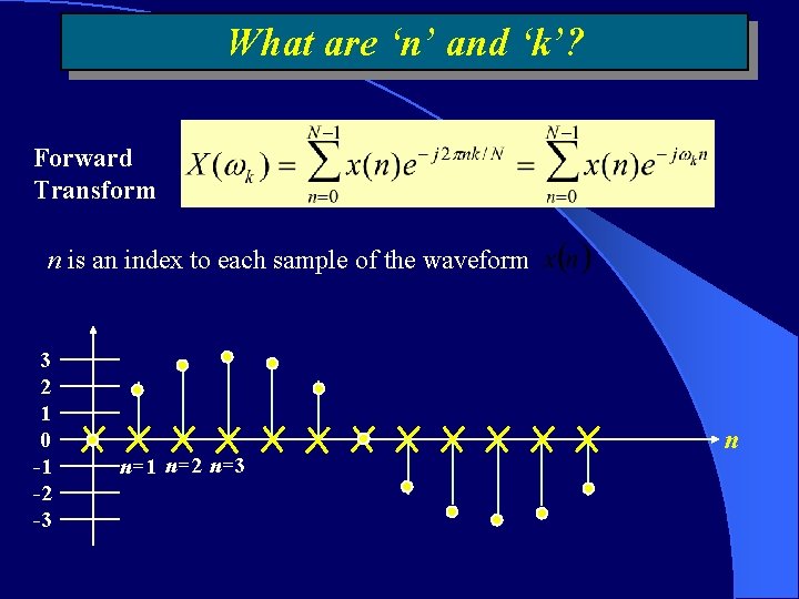
What are ‘n’ and ‘k’? Forward Transform n is an index to each sample of the waveform 3 2 1 0 -1 -2 -3 n=1 n=2 n=3 n

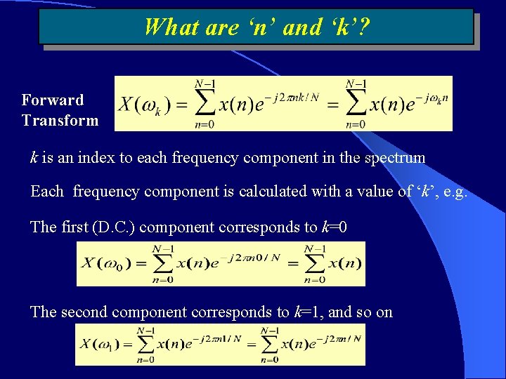
What are ‘n’ and ‘k’? Forward Transform k is an index to each frequency component in the spectrum Each frequency component is calculated with a value of ‘k’, e. g. The first (D. C. ) component corresponds to k=0 The second component corresponds to k=1, and so on

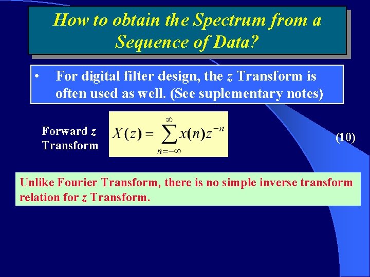
How to obtain the Spectrum from a Sequence of Data? • For digital filter design, the z Transform is often used as well. (See suplementary notes) Forward z Transform (10) Unlike Fourier Transform, there is no simple inverse transform relation for z Transform.

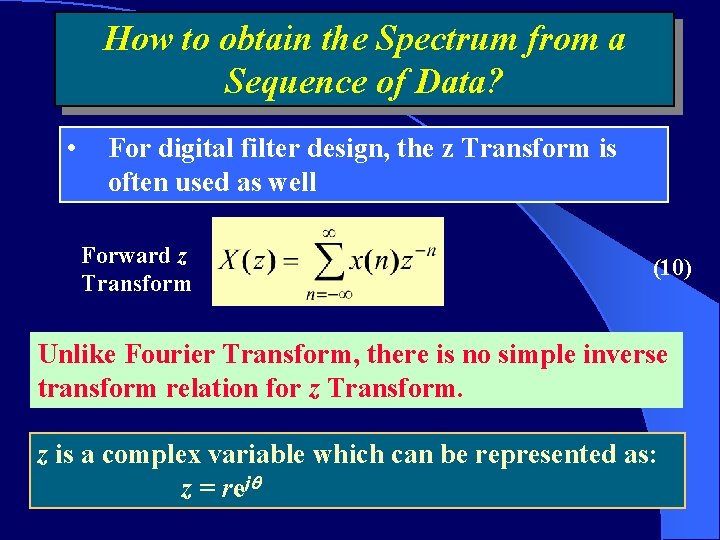
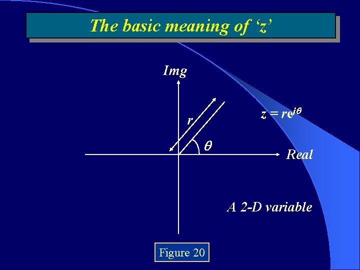
How to obtain the Spectrum from a Sequence of Data? • For digital filter design, the z Transform is often used as well Forward z Transform (10) Unlike Fourier Transform, there is no simple inverse transform relation for z Transform. z is a complex variable which can be represented as: z = rej

The basic meaning of ‘z’ Img z = rej r Real A 2 -D variable Figure 20