Microeconomics Supply and Demand Review The United States

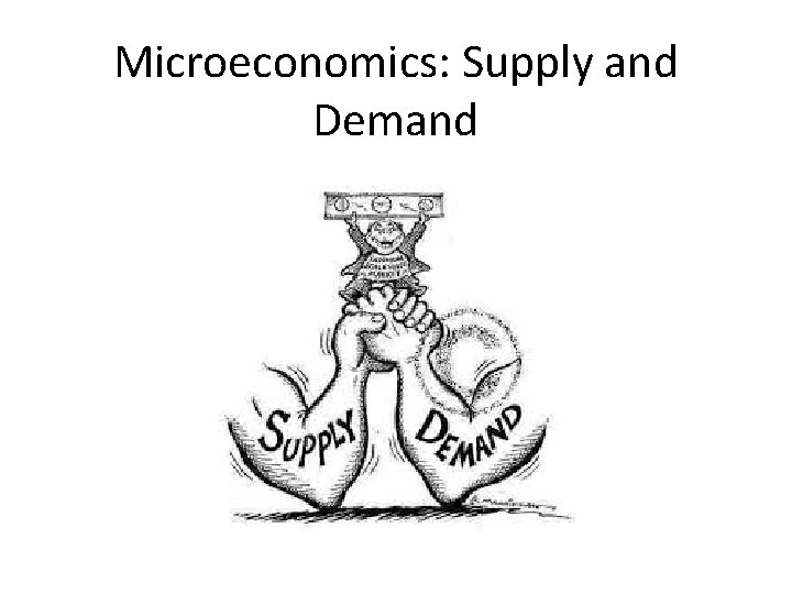
Microeconomics: Supply and Demand

Review The United States runs a mixed economy called Capitalism. This is closest to a market economy. The basic questions of economics are what, how and for whom to produce. In the Market economy these are all answered through individuals, and through supply and demand. The US practices Free Enterprise by limiting regulations of the economy to protect consumers and workers.

Microeconomics is the branch of economics that deals with the behavior and decision making by individual businesses and households. Micro-economists study concepts such as supply and demand, opening and closing of businesses and individual household budgets.

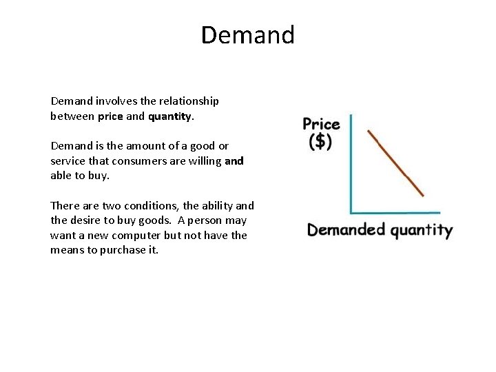
Demand involves the relationship between price and quantity. Demand is the amount of a good or service that consumers are willing and able to buy. There are two conditions, the ability and the desire to buy goods. A person may want a new computer but not have the means to purchase it.

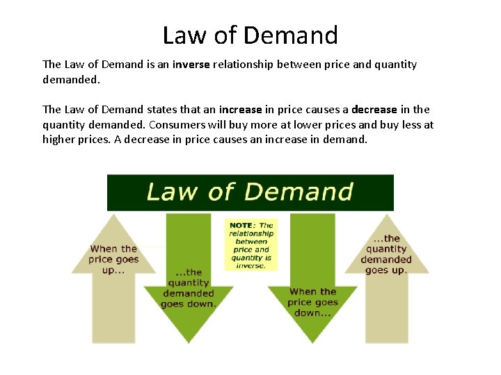
Law of Demand The Law of Demand is an inverse relationship between price and quantity demanded. The Law of Demand states that an increase in price causes a decrease in the quantity demanded. Consumers will buy more at lower prices and buy less at higher prices. A decrease in price causes an increase in demand. Law of Demand Price Demand or Price Demand

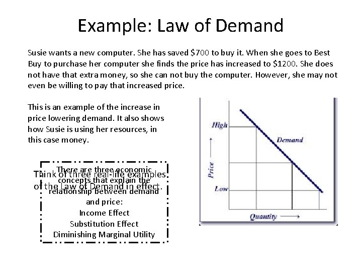
Example: Law of Demand Susie wants a new computer. She has saved $700 to buy it. When she goes to Best Buy to purchase her computer she finds the price has increased to $1200. She does not have that extra money, so she can not buy the computer. However, she may not even be willing to pay that increased price. This is an example of the increase in price lowering demand. It also shows how Susie is using her resources, in this case money. There are three economic Think of three real-life examples concepts that explain the of the Law of Demand effect. relationship betweenin demand price: Income Effect Substitution Effect Diminishing Marginal Utility

The Income Effect The amount of money, or income, that people have available to spend on goods and services is called their Purchasing Power An increase in a consumer’s purchasing power caused by a change in PRICE is called the Income Effect. The Income Effect says that when the price of a product goes down, people can afford to buy more of it. When the price goes up, people can’t buy as much. Example: If a person has $60 to spend on CDs but the price changes from $15 each to $10 each, their purchasing power has increased. Instead of being able to afford 4 CDs, they can now purchase 6 CDs.

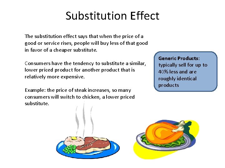
Substitution Effect The substitution effect says that when the price of a good or service rises, people will buy less of that good in favor of a cheaper substitute. Consumers have the tendency to substitute a similar, lower priced product for another product that is relatively more expensive. Example: the price of steak increases, so many consumers will switch to chicken, a lower priced substitute. Generic Products: typically sell for up to 40% less and are roughly identical products

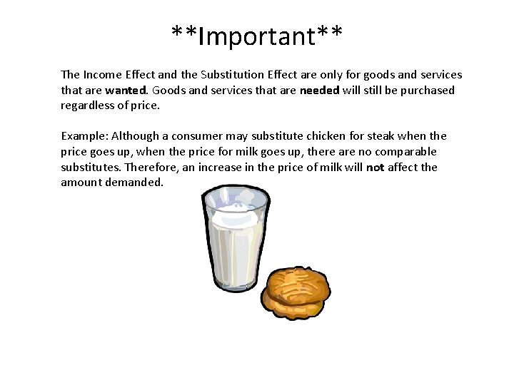
**Important** The Income Effect and the Substitution Effect are only for goods and services that are wanted. Goods and services that are needed will still be purchased regardless of price. Example: Although a consumer may substitute chicken for steak when the price goes up, when the price for milk goes up, there are no comparable substitutes. Therefore, an increase in the price of milk will not affect the amount demanded.

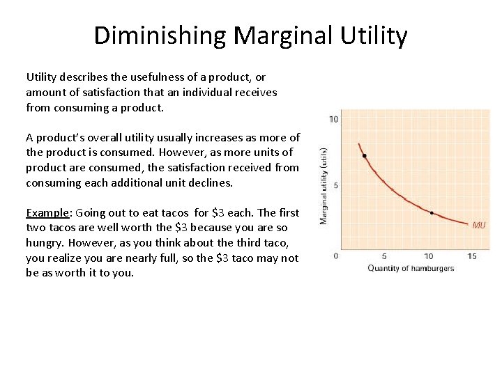
Diminishing Marginal Utility describes the usefulness of a product, or amount of satisfaction that an individual receives from consuming a product. A product’s overall utility usually increases as more of the product is consumed. However, as more units of product are consumed, the satisfaction received from consuming each additional unit declines. Example: Going out to eat tacos for $3 each. The first two tacos are well worth the $3 because you are so hungry. However, as you think about the third taco, you realize you are nearly full, so the $3 taco may not be as worth it to you.

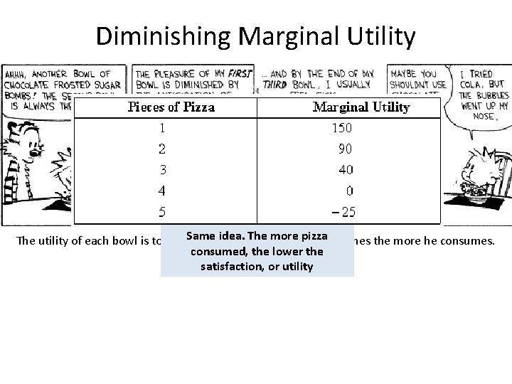
Diminishing Marginal Utility idea. more pizza The utility of each bowl is to feed. Same him but his. The satisfaction diminishes the more he consumes. consumed, the lower the satisfaction, or utility

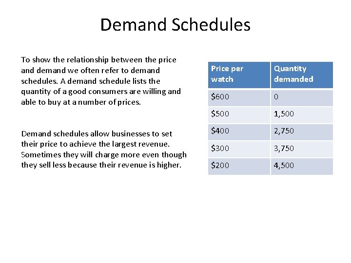
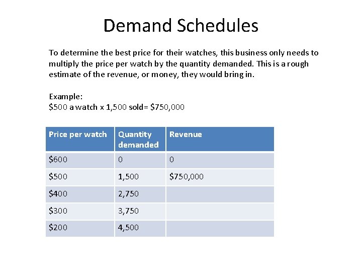
Demand Schedules To show the relationship between the price and demand we often refer to demand schedules. A demand schedule lists the quantity of a good consumers are willing and able to buy at a number of prices. Demand schedules allow businesses to set their price to achieve the largest revenue. Sometimes they will charge more even though they sell less because their revenue is higher. Price per watch Quantity demanded $600 0 $500 1, 500 $400 2, 750 $300 3, 750 $200 4, 500

Demand Schedules To determine the best price for their watches, this business only needs to multiply the price per watch by the quantity demanded. This is a rough estimate of the revenue, or money, they would bring in. Example: $500 a watch x 1, 500 sold= $750, 000 Price per watch Quantity demanded Revenue $600 0 0 $500 1, 500 $750, 000 $400 2, 750 $300 3, 750 $200 4, 500

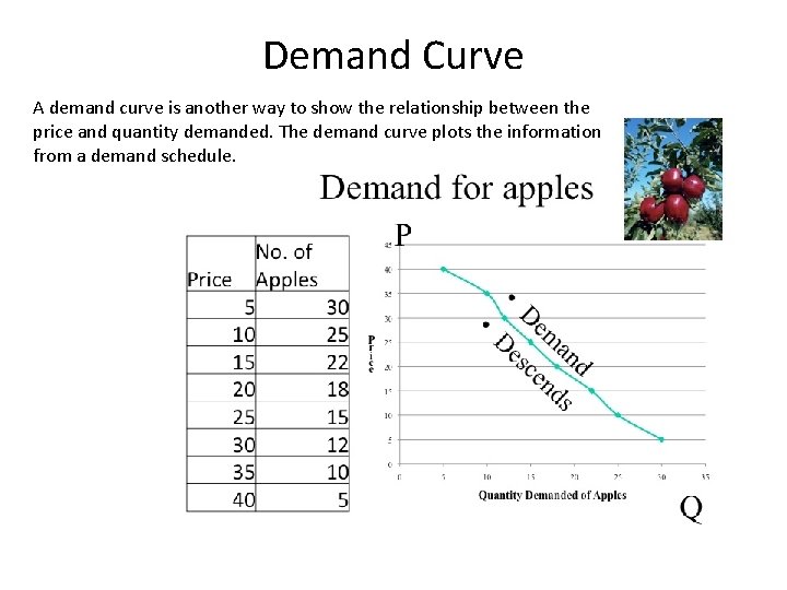
Demand Curve A demand curve is another way to show the relationship between the price and quantity demanded. The demand curve plots the information from a demand schedule.

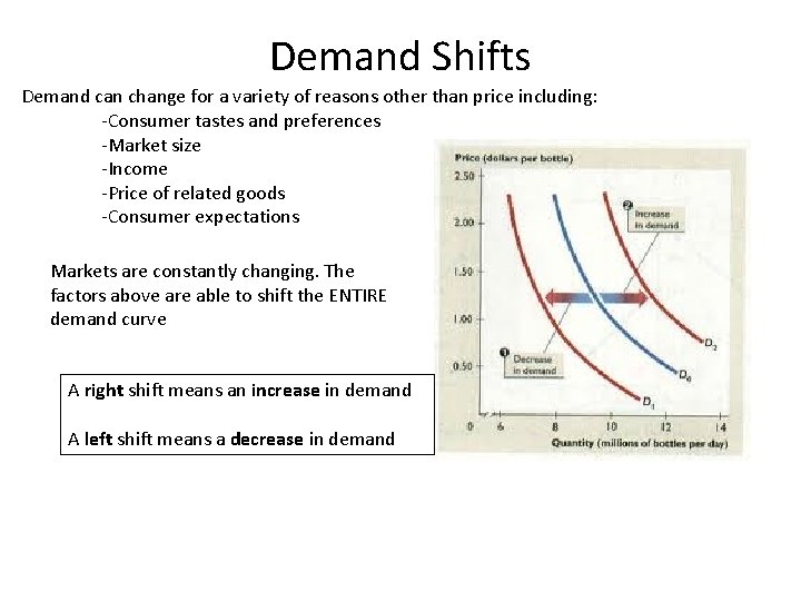
Demand Shifts Demand can change for a variety of reasons other than price including: -Consumer tastes and preferences -Market size -Income -Price of related goods -Consumer expectations Markets are constantly changing. The factors above are able to shift the ENTIRE demand curve A right shift means an increase in demand A left shift means a decrease in demand

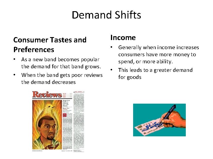
Demand Shifts Consumer Tastes and Preferences • As a new band becomes popular the demand for that band grows. • When the band gets poor reviews the demand decreases Income • Generally when income increases consumers have more money to spend, or more ability. • This leads to a greater demand for goods

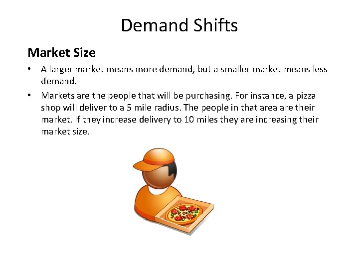
Demand Shifts Market Size • A larger market means more demand, but a smaller market means less demand. • Markets are the people that will be purchasing. For instance, a pizza shop will deliver to a 5 mile radius. The people in that area are their market. If they increase delivery to 10 miles they are increasing their market size.

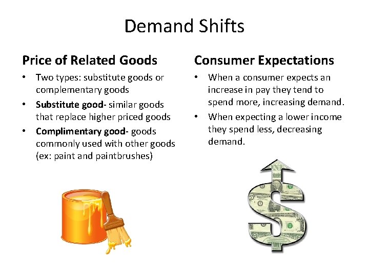
Demand Shifts Price of Related Goods Consumer Expectations • Two types: substitute goods or complementary goods • Substitute good- similar goods that replace higher priced goods • Complimentary good- goods commonly used with other goods (ex: paint and paintbrushes) • When a consumer expects an increase in pay they tend to spend more, increasing demand. • When expecting a lower income they spend less, decreasing demand.

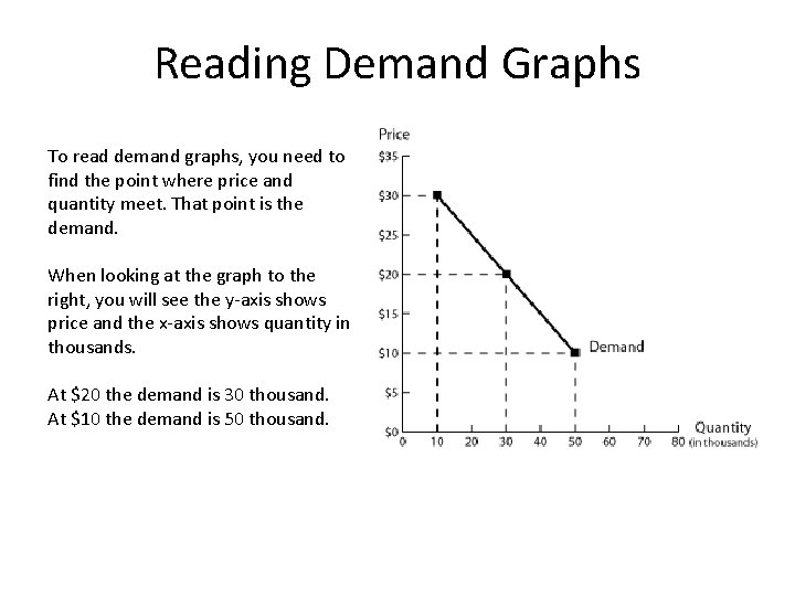
Reading Demand Graphs To read demand graphs, you need to find the point where price and quantity meet. That point is the demand. When looking at the graph to the right, you will see the y-axis shows price and the x-axis shows quantity in thousands. At $20 the demand is 30 thousand. At $10 the demand is 50 thousand.

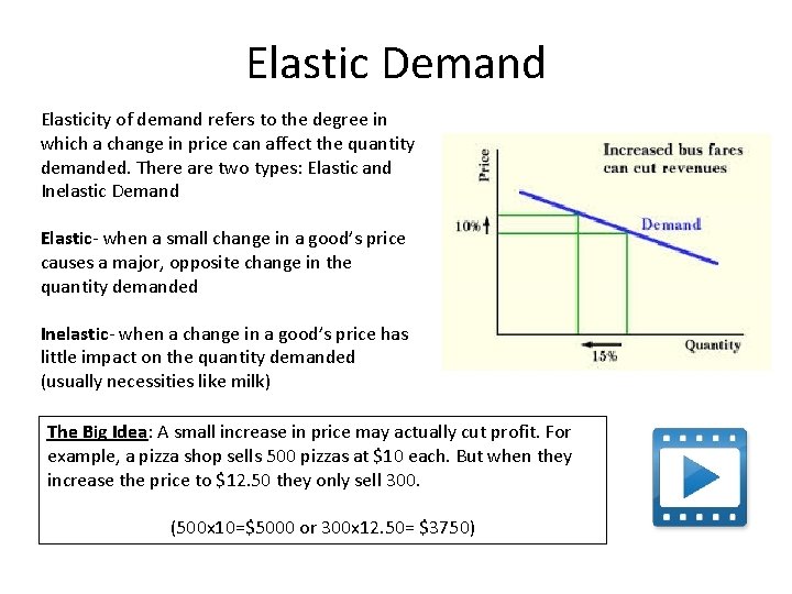
Elastic Demand Elasticity of demand refers to the degree in which a change in price can affect the quantity demanded. There are two types: Elastic and Inelastic Demand Elastic- when a small change in a good’s price causes a major, opposite change in the quantity demanded Inelastic- when a change in a good’s price has little impact on the quantity demanded (usually necessities like milk) The Big Idea: A small increase in price may actually cut profit. For example, a pizza shop sells 500 pizzas at $10 each. But when they increase the price to $12. 50 they only sell 300. (500 x 10=$5000 or 300 x 12. 50= $3750)

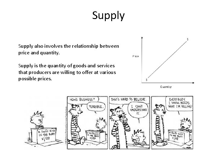
Supply also involves the relationship between price and quantity. Supply is the quantity of goods and services that producers are willing to offer at various possible prices.

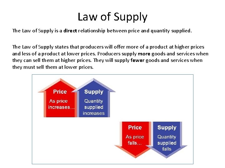
Law of Supply The Law of Supply is a direct relationship between price and quantity supplied. The Law of Supply states that producers will offer more of a product at higher prices and less of a product at lower prices. Producers supply more goods and services when they can sell them at higher prices. They will supply fewer goods and services when they must sell them at lower prices.

Profit The amount of money remaining after producers have paid all of their costs is called profit. Businesses make money when revenues (incoming money) are greater than the costs of production. Businesses take risks and make decisions based on profits. They rely on supply schedules and supply curves to make decisions on what, how and for whom to produce.

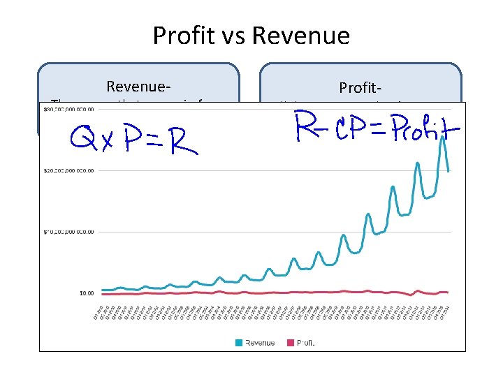
Profit vs Revenue- The money that comes in from selling goods and services Profit- All the money made after costs The goal of capitalist businesses is to maximize profit. Businesses do this in a number ways: -increasing price of product -using cheaper supplies -reducing amount in packaged products

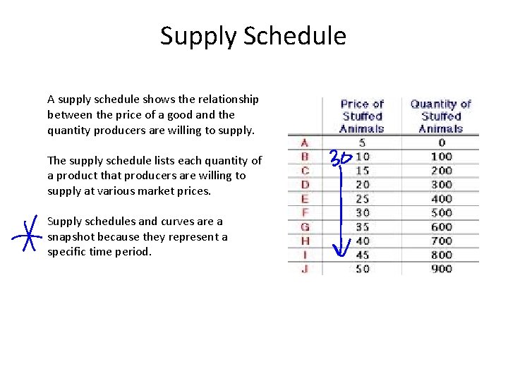
Supply Schedule A supply schedule shows the relationship between the price of a good and the quantity producers are willing to supply. The supply schedule lists each quantity of a product that producers are willing to supply at various market prices. Supply schedules and curves are a snapshot because they represent a specific time period.

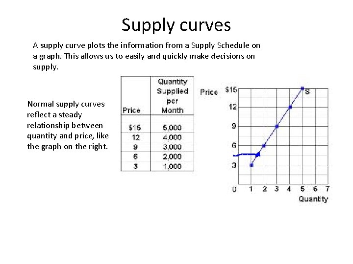
Supply curves A supply curve plots the information from a Supply Schedule on a graph. This allows us to easily and quickly make decisions on supply. Normal supply curves reflect a steady relationship between quantity and price, like the graph on the right.

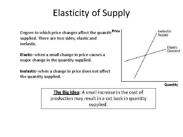
Elasticity of Supply Degree to which price changes affect the quantity supplied. There are two sides, elastic and inelastic. Elastic- when a small change in price causes a major change in the quantity supplied. Inelastic- when a change in price does not affect the quantity supplied. The Big Idea: A small increase in the cost of production may result in a cut back in quantity supplied.

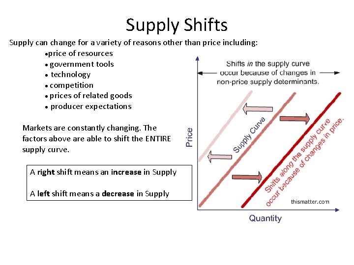
Supply Shifts Supply can change for a variety of reasons other than price including: ●price of resources ● government tools ● technology ● competition ● prices of related goods ● producer expectations Markets are constantly changing. The factors above are able to shift the ENTIRE supply curve. A right shift means an increase in Supply A left shift means a decrease in Supply

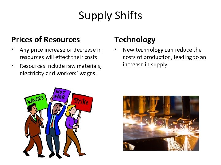
Supply Shifts Prices of Resources Technology • Any price increase or decrease in resources will effect their costs • Resources include raw materials, electricity and workers’ wages. • New technology can reduce the costs of production, leading to an increase in supply

Supply Shifts Government tools • Tools include taxes, subsidies and regulation, which can change how much a company is willing to produce • Taxes: payment to fund government services. Taxes add to cost of production • Subsidies: payments to private businesses to ensure an affordable supply of some essential goods like dairy, wheat, etc. – Example- Corn-vs-Wheat • Regulations: rules on how a business can operate which are meant to protect the consumer – Example- Coca-Cola

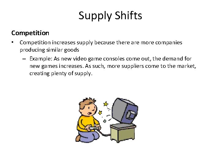
Supply Shifts Competition • Competition increases supply because there are more companies producing similar goods – Example: As new video game consoles come out, the demand for new games increases. As such, more suppliers come to the market, creating plenty of supply.

Supply Shifts Prices of Related Goods Producer Expectations • Suppliers may choose to produce different goods which are selling for a higher profit • Example: farmer growing wheat will want to switch to growing corn if the price of corn goes up • If the producers think the demand for or the price of their products will increase they will increase their supply

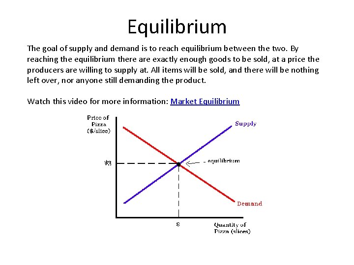
Equilibrium The goal of supply and demand is to reach equilibrium between the two. By reaching the equilibrium there are exactly enough goods to be sold, at a price the producers are willing to supply at. All items will be sold, and there will be nothing left over, nor anyone still demanding the product. Watch this video for more information: Market Equilibrium

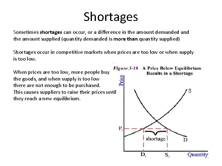
Shortages Sometimes shortages can occur, or a difference in the amount demanded and the amount supplied (quantity demanded is more than quantity supplied) Shortages occur in competitive markets when prices are too low or when supply is too low. When prices are too low, more people buy the goods, and when supply is too low there are not enough to be purchased. This causes suppliers to raise their prices until they reach a new equilibrium.

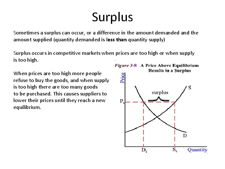
Surplus Sometimes a surplus can occur, or a difference in the amount demanded and the amount supplied (quantity demanded is less than quantity supply) Surplus occurs in competitive markets when prices are too high or when supply is too high. When prices are too high more people refuse to buy the goods, and when supply is too high there are too many goods to be purchased. This causes suppliers to lower their prices until they reach a new equilibrium.

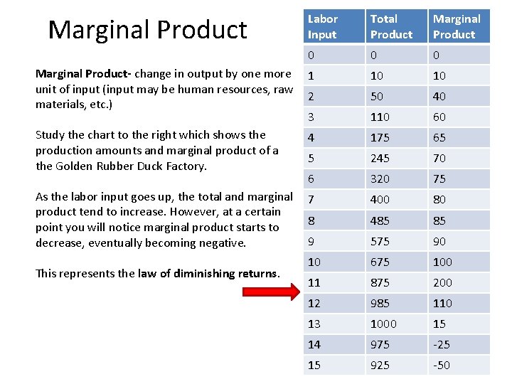
Making Production Decisions are made based on productivity-how many goods or services can be produced per unit of input. Producers want to make the greatest total output- amount produced in a given period of time with current resources and input. Once total output is calculated the producers also determine their marginal outputthe change in output by adding one more unit of input.

Labor Input Total Product Marginal Product 0 0 0 Marginal Product- change in output by one more unit of input (input may be human resources, raw materials, etc. ) 1 10 10 2 50 40 3 110 60 Study the chart to the right which shows the production amounts and marginal product of a the Golden Rubber Duck Factory. 4 175 65 5 245 70 6 320 75 As the labor input goes up, the total and marginal product tend to increase. However, at a certain point you will notice marginal product starts to decrease, eventually becoming negative. 7 400 80 8 485 85 9 575 90 10 675 100 11 875 200 12 985 110 13 1000 15 14 975 -25 15 925 -50 Marginal Product This represents the law of diminishing returns.

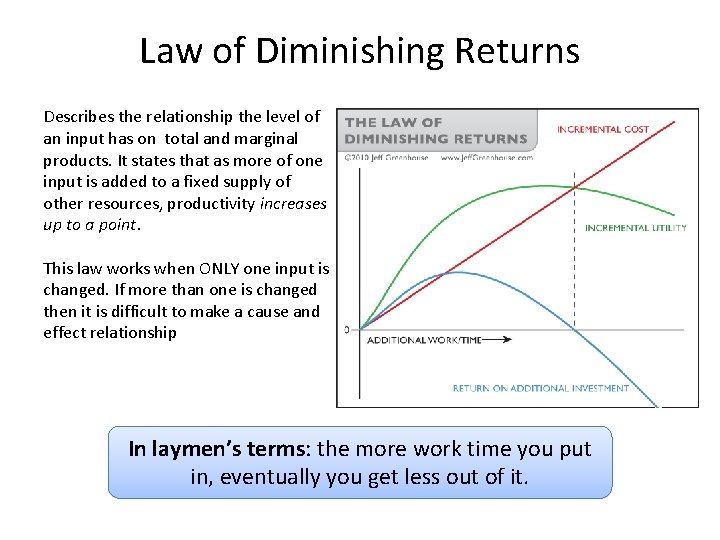
Law of Diminishing Returns Describes the relationship the level of an input has on total and marginal products. It states that as more of one input is added to a fixed supply of other resources, productivity increases up to a point. This law works when ONLY one input is changed. If more than one is changed then it is difficult to make a cause and effect relationship In laymen’s terms: the more work time you put in, eventually you get less out of it.

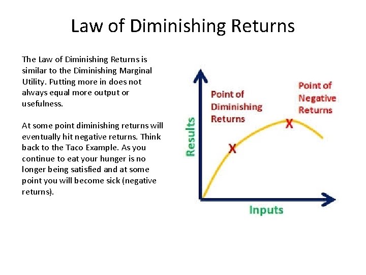
Law of Diminishing Returns The Law of Diminishing Returns is similar to the Diminishing Marginal Utility. Putting more in does not always equal more output or usefulness. At some point diminishing returns will eventually hit negative returns. Think back to the Taco Example. As you continue to eat your hunger is no longer being satisfied and at some point you will become sick (negative returns).

Costs of Production Producers also examine their costs of production to determine the best amount of goods to supply. Costs include any goods and services used to make a product. There are several categories of production costs: 1) 2) 3) 4) Fixed Variable Total Marginal costs

Fixed Costs Some production costs do not change, no matter how many goods are made. These are known as fixed costs. Examples of fixed costs include rent, interest on loans, property insurance, property taxes and salaries. Big Idea: Even if the Golden Duck factory makes zero ducks, they still owe rent, taxes and other fixed costs.

Variable Costs These are costs that change as the level of output changes. These include raw materials and wages. For example, the Golden Duck factory raises production from 100 ducks to 1000 a day. The cost of production will go up because the factory must pay more workers and buy more raw materials.

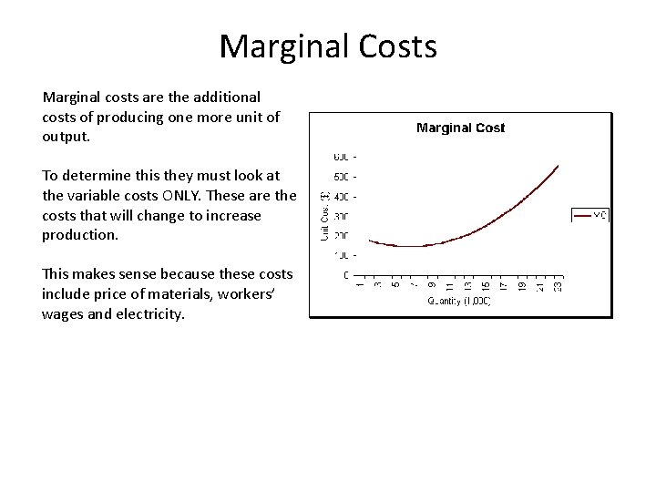
Marginal Costs Marginal costs are the additional costs of producing one more unit of output. To determine this they must look at the variable costs ONLY. These are the costs that will change to increase production. This makes sense because these costs include price of materials, workers’ wages and electricity.

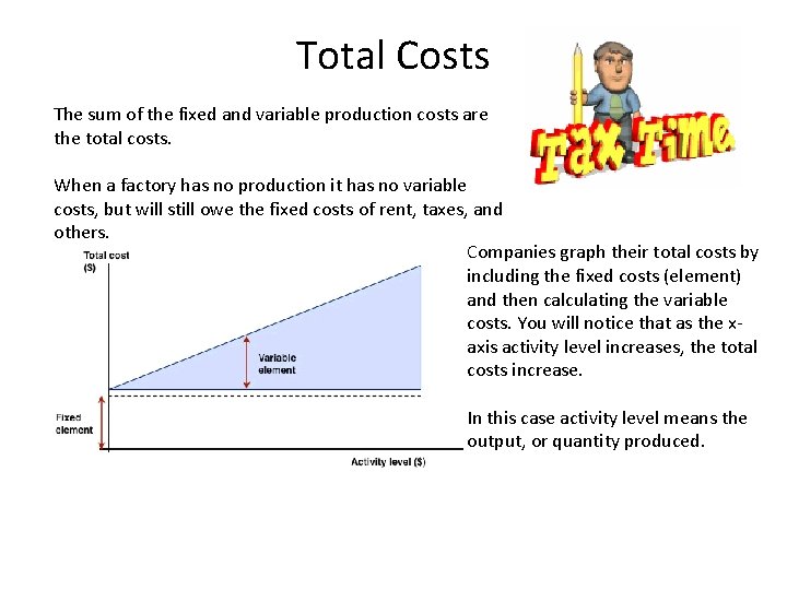
Total Costs The sum of the fixed and variable production costs are the total costs. When a factory has no production it has no variable costs, but will still owe the fixed costs of rent, taxes, and others. Companies graph their total costs by including the fixed costs (element) and then calculating the variable costs. You will notice that as the xaxis activity level increases, the total costs increase. In this case activity level means the output, or quantity produced.

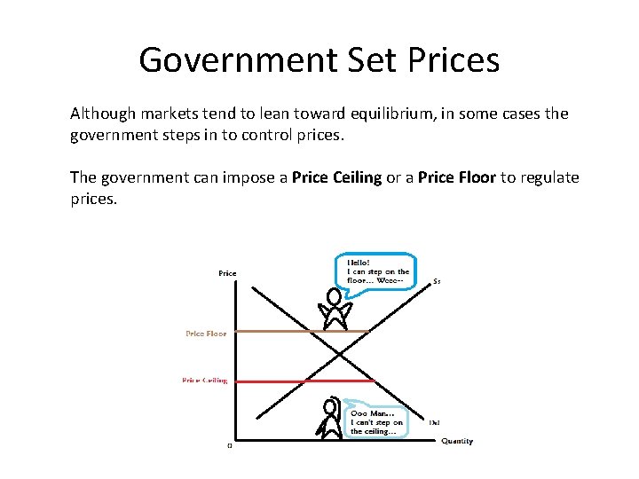
Government Set Prices Although markets tend to lean toward equilibrium, in some cases the government steps in to control prices. The government can impose a Price Ceiling or a Price Floor to regulate prices.

Price Ceilings • A price ceiling is a maximum price that can legally be charged for a good. The price is artificially held below the equilibrium price and is not allowed to rise. – Who benefits from this? • The government places price ceilings on some goods that are considered “essential” and might become too expensive for consumers. • Because these price ceilings are set below equilibrium, they end up causing shortages (more demand than supply)

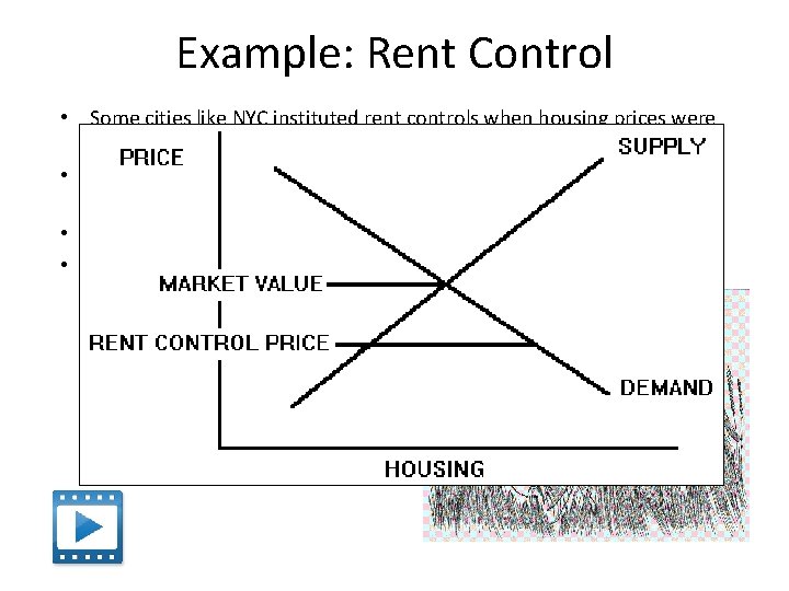
Example: Rent Control • Some cities like NYC instituted rent controls when housing prices were rising rapidly and current city residents could no longer afford rent • Rent is only allowed to rise a certain percentage each year, but stays below equilibrium • Price ceilings provide a gain for buyers and a loss for sellers • Has resulted in a shortage of apartments because they require owners to accept a price that is lower than the equilibrium price. Rather than accept the low price, owner often convert the apartments to condominiums and sell them, decreasing the supply of available apartments

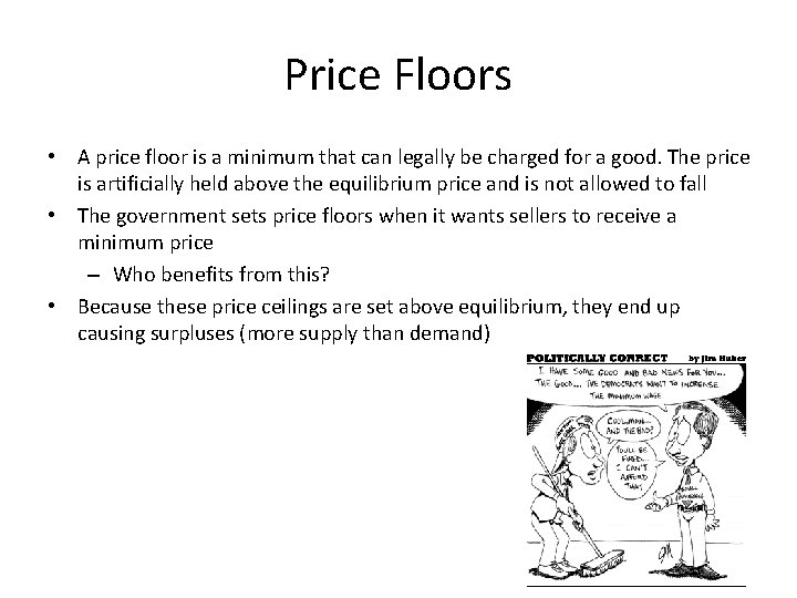
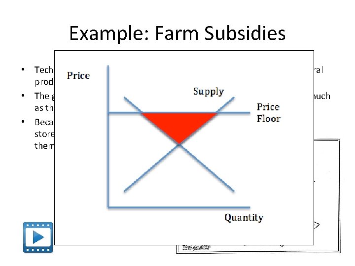
Price Floors • A price floor is a minimum that can legally be charged for a good. The price is artificially held above the equilibrium price and is not allowed to fall • The government sets price floors when it wants sellers to receive a minimum price – Who benefits from this? • Because these price ceilings are set above equilibrium, they end up causing surpluses (more supply than demand)

Example: Farm Subsidies • Technological advances have greatly increased the supply of agricultural products, but demand has increased much less. • The government sets a price floor that allows farmers to produce as much as they want to sell at a set price. • Because there’s a shortage, the government will buy excess crops and store them, sell them, or give them away