Maximum Likelihood Estimation and Simplified Kalman Filter tecniques

Basic concepts State vector : atmospheric state of the forecast model True state :

Modelling of errors Background unbiased error: Background error’s covariance matrix: Observation unbiased error: Observation

The Kalman Filter Equations for the analysis and propagation of the model state for

On line estimation of covariance parameters • Maximum likelihood approach suggested by Dee for

Maximum likelihood method We parametrize the aspected value of the innovation as follows We

Application to HIRVDA Data • Selected observational data for each type of observations •

Estimations of statistics for observations and model errors Assuming the following conditions: • The

Slides: 8

Download presentation

Maximum Likelihood Estimation and Simplified Kalman Filter tecniques for real time Data Assimilation

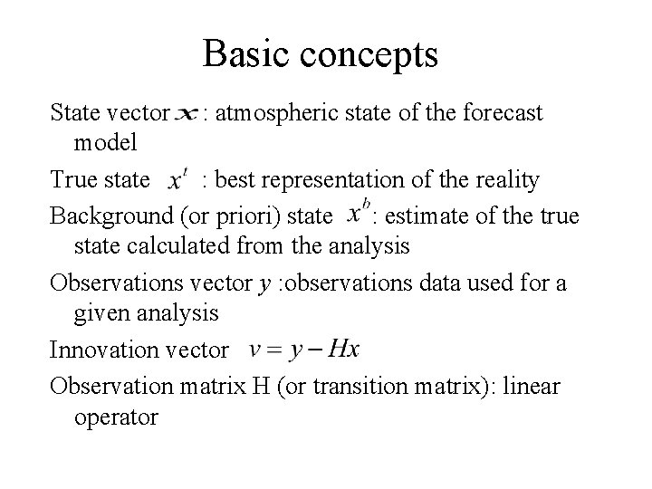
Basic concepts State vector : atmospheric state of the forecast model True state : best representation of the reality Background (or priori) state : estimate of the true state calculated from the analysis Observations vector y : observations data used for a given analysis Innovation vector Observation matrix H (or transition matrix): linear operator

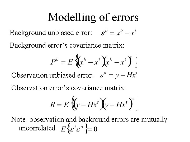
Modelling of errors Background unbiased error: Background error’s covariance matrix: Observation unbiased error: Observation error’s covariance matrix: Note: observation and backround errors are mutually uncorrelated

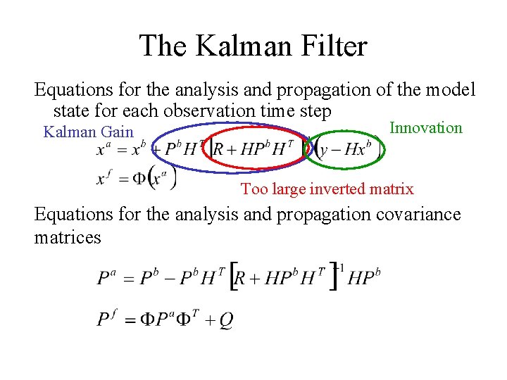
The Kalman Filter Equations for the analysis and propagation of the model state for each observation time step Kalman Gain Innovation Too large inverted matrix Equations for the analysis and propagation covariance matrices

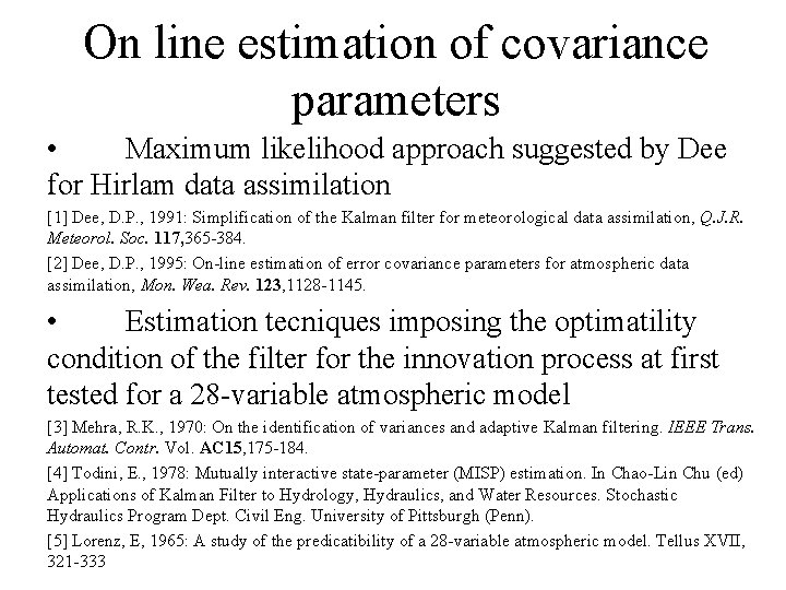
On line estimation of covariance parameters • Maximum likelihood approach suggested by Dee for Hirlam data assimilation [1] Dee, D. P. , 1991: Simplification of the Kalman filter for meteorological data assimilation, Q. J. R. Meteorol. Soc. 117, 365 -384. [2] Dee, D. P. , 1995: On-line estimation of error covariance parameters for atmospheric data assimilation, Mon. Wea. Rev. 123, 1128 -1145. • Estimation tecniques imposing the optimatility condition of the filter for the innovation process at first tested for a 28 -variable atmospheric model [3] Mehra, R. K. , 1970: On the identification of variances and adaptive Kalman filtering. IEEE Trans. Automat. Contr. Vol. AC 15, 175 -184. [4] Todini, E. , 1978: Mutually interactive state-parameter (MISP) estimation. In Chao-Lin Chu (ed) Applications of Kalman Filter to Hydrology, Hydraulics, and Water Resources. Stochastic Hydraulics Program Dept. Civil Eng. University of Pittsburgh (Penn). [5] Lorenz, E, 1965: A study of the predicatibility of a 28 -variable atmospheric model. Tellus XVII, 321 -333

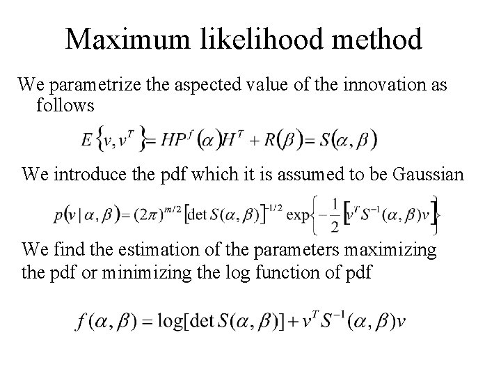
Maximum likelihood method We parametrize the aspected value of the innovation as follows We introduce the pdf which it is assumed to be Gaussian We find the estimation of the parameters maximizing the pdf or minimizing the log function of pdf

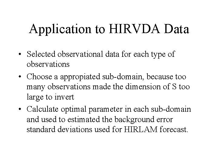
Application to HIRVDA Data • Selected observational data for each type of observations • Choose a appropiated sub-domain, because too many observations made the dimension of S too large to invert • Calculate optimal parameter in each sub-domain and used to estimated the background error standard deviations used for HIRLAM forecast.

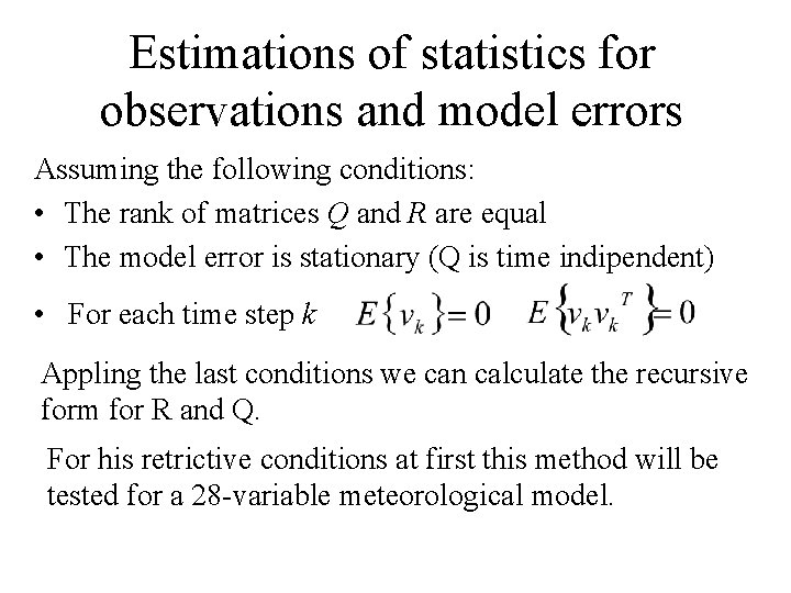
Estimations of statistics for observations and model errors Assuming the following conditions: • The rank of matrices Q and R are equal • The model error is stationary (Q is time indipendent) • For each time step k Appling the last conditions we can calculate the recursive form for R and Q. For his retrictive conditions at first this method will be tested for a 28 -variable meteorological model.