Matrix Operator scaling and their many applications Avi

Matrix & Operator scaling and their many applications Avi Wigderson IAS, Princeton based on joint works with Ankit Garg, Leonid Gurvits and Rafael Olivera

Matrix scaling applications Numerical analysis Making linear systems numerically stable Signal processing CAT scans, … Approximating the permanent Deterministically! Combinatorial geometry Incidence theorems

Operator scaling applications Non-commutative Algebra Word problem in free skew fields Invariant Theory Nullcone membership for Left-Right action Quantum Information Theory Rank decrease of completely positive operators Analysis Brascamp-Lieb inequalities Computational complexity (? ) PIT, Rank of symbolic matrices, lower bounds Optimization (? ) Solving certain general families of - Quadratic systems of equations - Exponentially large linear programs

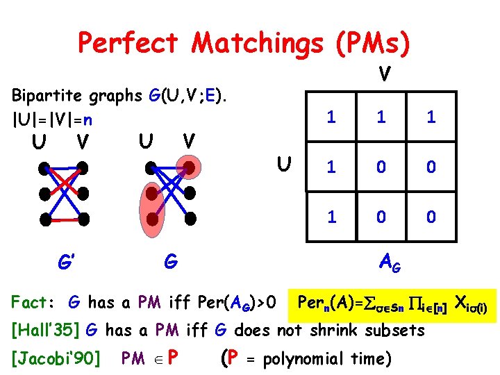
Perfect Matchings (PMs) V Bipartite graphs G(U, V; E). |U|=|V|=n U V G’ U V U 1 1 0 0 AG G Fact: G has a PM iff Per(AG)>0 Pern(A)= Sn i [n] Xi (i) [Hall’ 35] G has a PM iff G does not shrink subsets [Jacobi‘ 90] PM P (P = polynomial time)

PMs & symbolic matrices U V G [Edmonds‘ 67] 1 1 1 x 12 x 13 1 0 0 x 21 0 0 x 31 0 0 AG AG(X) [Edmonds ‘ 67] G has a PM iff Det(AG(X)) 0 ( P)

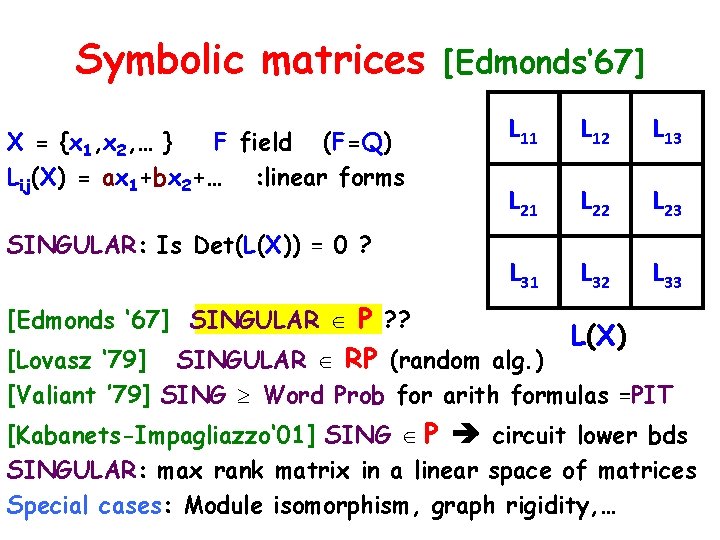
Symbolic matrices X = {x 1, x 2, … } F field (F=Q) Lij(X) = ax 1+bx 2+… : linear forms SINGULAR: Is Det(L(X)) = 0 ? [Edmonds ‘ 67] SINGULAR P ? ? [Edmonds‘ 67] L 11 L 12 L 13 L 21 L 22 L 23 L 31 L 32 L 33 L(X) [Lovasz ‘ 79] SINGULAR RP (random alg. ) [Valiant ’ 79] SING Word Prob for arith formulas =PIT [Kabanets-Impagliazzo‘ 01] SING P circuit lower bds SINGULAR: max rank matrix in a linear space of matrices Special cases: Module isomorphism, graph rigidity, …

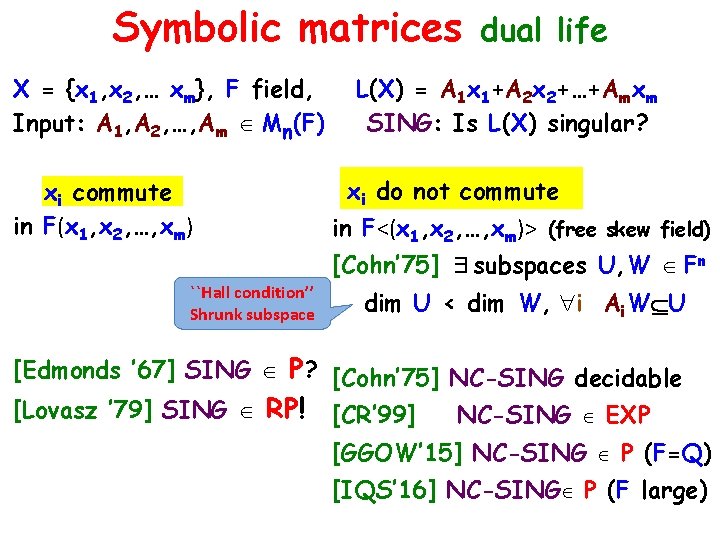
Symbolic matrices X = {x 1, x 2, … xm}, F field, Input: A 1, A 2, …, Am Mn(F) xi commute in F(x 1, x 2, …, xm) dual life L(X) = A 1 x 1+A 2 x 2+…+Amxm SING: Is L(X) singular? xi do not commute in F<(x 1, x 2, …, xm)> (free skew field) [Cohn’ 75] ∃subspaces U, W Fn ``Hall condition’’ Shrunk subspace dim U < dim W, i Ai. W U [Edmonds ’ 67] SING P? [Cohn’ 75] NC-SING decidable [Lovasz ’ 79] SING RP! [CR’ 99] NC-SING EXP [GGOW’ 15] NC-SING P (F=Q) [IQS’ 16] NC-SING P (F large)

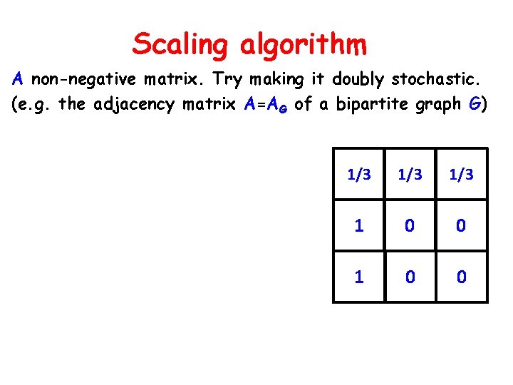
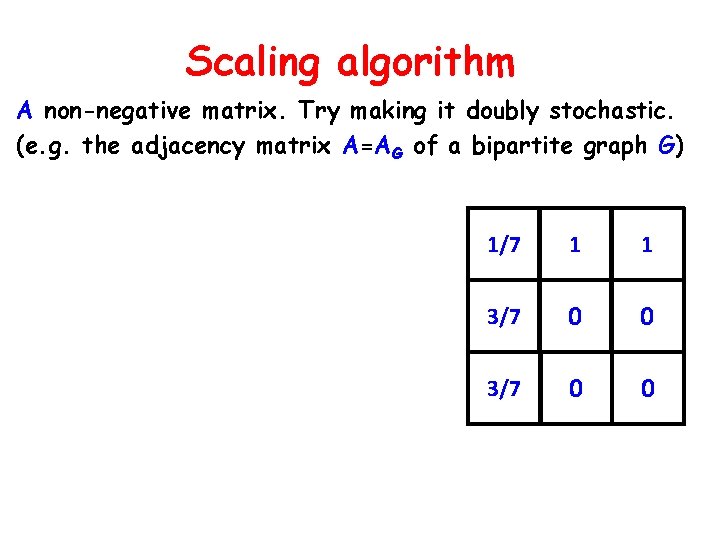
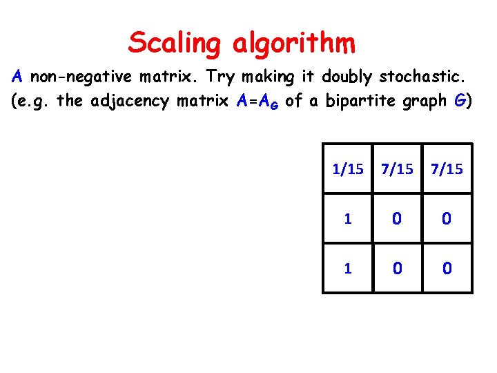
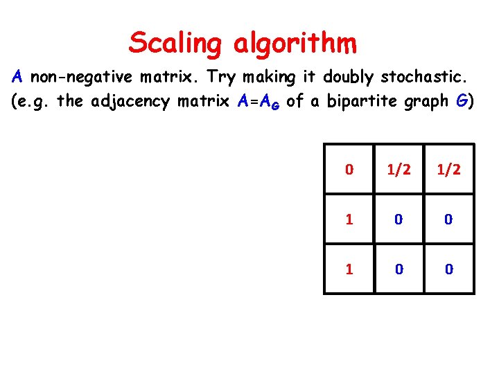
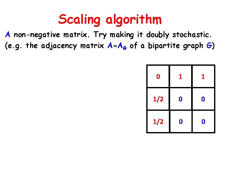
Matrix scaling algorithm [Sinkhorn’ 64, LSW’ 01, GY’ 03] A non-negative matrix. Try making it doubly stochastic. (e. g. the adjacency matrix A=AG of a bipartite graph G) Allowed: Multiply rows & columns by scalars Find (if exists? ) R, C diagonal s. t. RAC has row-sums & col-sums =1 1 1 0 0 [Sinkhorn’ 64] Just do it! First rows, then columns…

Scaling algorithm A non-negative matrix. Try making it doubly stochastic. (e. g. the adjacency matrix A=AG of a bipartite graph G) 1/3 1/3 1 0 0

Scaling algorithm A non-negative matrix. Try making it doubly stochastic. (e. g. the adjacency matrix A=AG of a bipartite graph G) 1/7 1 1 3/7 0 0

Scaling algorithm A non-negative matrix. Try making it doubly stochastic. (e. g. the adjacency matrix A=AG of a bipartite graph G) 1/15 7/15 1 0 0

Scaling algorithm A non-negative matrix. Try making it doubly stochastic. (e. g. the adjacency matrix A=AG of a bipartite graph G) 0 1 1 1/2 0 0

Scaling algorithm A non-negative matrix. Try making it doubly stochastic. (e. g. the adjacency matrix A=AG of a bipartite graph G) 0 1/2 1 0 0

Scaling algorithm A non-negative matrix. Try making it doubly stochastic. (e. g. the adjacency matrix A=AG of a bipartite graph G) 0 1 1 1/2 0 0

Scaling algorithm A non-negative matrix. Try making it doubly stochastic. (e. g. the adjacency matrix A=AG of a bipartite graph G) 0 1/2 1 0 0

Scaling algorithm [LSW ‘ 01] A non-negative matrix. Try making it doubly stochastic. (e. g. the adjacency matrix A=AG of a bipartite graph G) R(A) = diag(row sums)-1 C(A) = diag(column sums)-1 Repeat n 3 times: Normalize rows A �R(A) A Normalize cols A �A C(A) 1 1 1 0 0

Scaling algorithm [LSW ‘ 01] A non-negative matrix. Try making it doubly stochastic. (e. g. the adjacency matrix A=AG of a bipartite graph G) R(A) = diag(row sums)-1 C(A) = diag(column sums)-1 Repeat n 3 times: Normalize rows A �R(A) A Normalize cols A �A C(A) 1/3 1/3 1/2 0 1 0 0

Scaling algorithm [LSW ‘ 01] A non-negative matrix. Try making it doubly stochastic. (e. g. the adjacency matrix A=AG of a bipartite graph G) R(A) = diag(row sums)-1 C(A) = diag(column sums)-1 Repeat n 3 times: Normalize rows A �R(A) A Normalize cols A �A C(A) 2/11 2/5 1 3/11 3/5 0 6/11 0 0

Scaling algorithm [LSW ‘ 01] A non-negative matrix. Try making it doubly stochastic. (e. g. the adjacency matrix A=AG of a bipartite graph G) R(A) = diag(row sums)-1 C(A) = diag(column sums)-1 Repeat n 3 times: Normalize rows A �R(A) A Normalize cols A �A C(A) 10/87 22/87 55/87 15/48 33/48 1 0 0 0

Scaling algorithm [LSW ‘ 01] A non-negative (0, 1) matrix. “Make it doubly stochastic” (e. g. the adjacency matrix A=AG of a bipartite graph G) R(A) = diag(row sums)-1 C(A) = diag(column sums)-1 Repeat n 3 times: Normalize rows A �R(A) A Normalize cols A �A C(A) (C(A)=I) Test if R(A) I (up to 1/n) Yes: Per(A) > 0. No: Per(A) = 0. Analysis: - 0 0 1 0 1 0 0 Per(A)>0 Per(A)>exp(-n) (easy) Per(A) grows by (1+1/n) (AMGM) Per(A) ≤ 1 |R(A)-I|< 1/n Per(A) >0 (Cauchy-Schwarz)

Operator scaling algorithm [Gurvits ’ 04, GGOW’ 15] L=(A 1, A 2, …, Am). Try making it “doubly stochastic” i. Ait=I i. Ait. Ai=I. Allowed: L RLC, R(L) = ( i. Ait)-1/2 C(L) = ( i. Ait. Ai)-1/2 Repeat nc times: Normalize rows L �R(L) L Normalize cols L �L C(L) Test if C(L) I (up to 1/n) Yes: L NC-nonsingular No: L NC-singular R, C invertible Invertible [GGOW’ 15] - NC-rank P - Computes Cap(L) & scaling factors - Alg continuous in L Analysis: Cap(L)>0 Cap(L)>exp(-n) [GGOW’ 15] Cap(L) grows by (1+1/n) (AMGM) Cap(L) ≤ 1 |R(L)-I|< 1/n Cap(A) 1 (Cauchy-Schwarz)

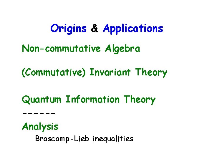
Origins & Applications Non-commutative Algebra (Commutative) Invariant Theory Quantum Information Theory -----Analysis Brascamp-Lieb inequalities

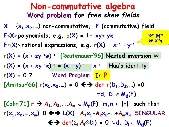
Non-commutative algebra Word problem for free skew fields X = {x 1, x 2, …} non-commutative, F (commutative) field F<X> polynomials, e. g. p(X) = 1+ xy+ yx F<(X)> rational expressions, e. g. r(X) = x-1 + y-1 not pq-1 or p-1 q r(X) = (x + zy-1 w)-1 [Reutenauer’ 96] Nested inversion ∞ r(X) = (x + xy-1 x)-1 = (x + y)-1 - x-1 r(X) = 0 ? Hua’s identity Word Problem In P [Amitsur’ 66] r(x 1, x 2, …) = 0 det r(D 1, D 2, …) =0 d, Di Md(F) [Cohn’ 71] r A 1, A 2, …, Am Mn(F) m, n ≤ |r| such that r(x 1, x 2, …, xm)=0 L(X)= A 1 x 1+A 2 x 2+…+Amxm SINGULAR det( i Ai Di) = 0 d, Di Md(F)

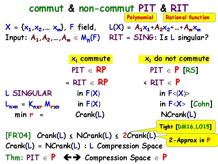
commut & non-commut PIT & RIT Polynomial X = {x 1, x 2, … xm}, F field, Input: A 1, A 2, …, Am Mn(F) L(X) = A 1 x 1+A 2 x 2+…+Amxm RIT = SING: Is L singular? xi commute PIT RP L SINGULAR Lnxn = Knxr Mrxn min r = = RIT RP in F(X) Crank(L) Rational function xi do not commute PIT P [RS] < RIT P in F<(X)> in F<X> [Cohn] NCrank(L) Tight [DM 16, LO 15] [FR’ 04] Crank(L) ≤ NCrank(L) ≤ 2 Crank(L) 2 -Approx in P Crank(L) = NCrank(L) : L Compression Space Thm: PIT P Compression Space P

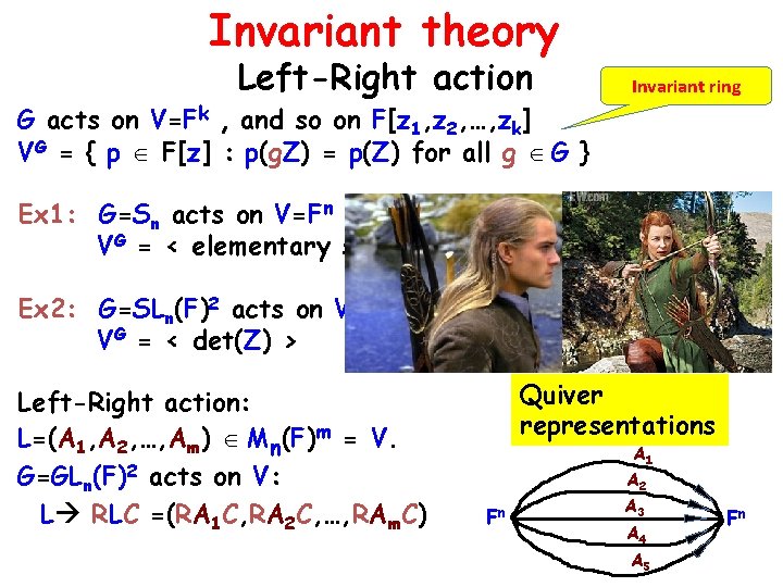
Invariant theory Left-Right action G acts on V=Fk , and so on F[z 1, z 2, …, zk] VG = { p F[z] : p(g. Z) = p(Z) for all g G } Invariant ring Ex 1: G=Sn acts on V=Fn by permuting coordinates VG = < elementary symmetric polynomials > Ex 2: G=SLn(F)2 acts on V=Mn(F) VG = < det(Z) > Left-Right action: L=(A 1, A 2, …, Am) Mn(F)m = V. G=GLn(F)2 acts on V: L RLC =(RA 1 C, RA 2 C, …, RAm. C) by Z RZC Quiver representations A 1 Fn A 2 A 3 A 4 A 5 Fn

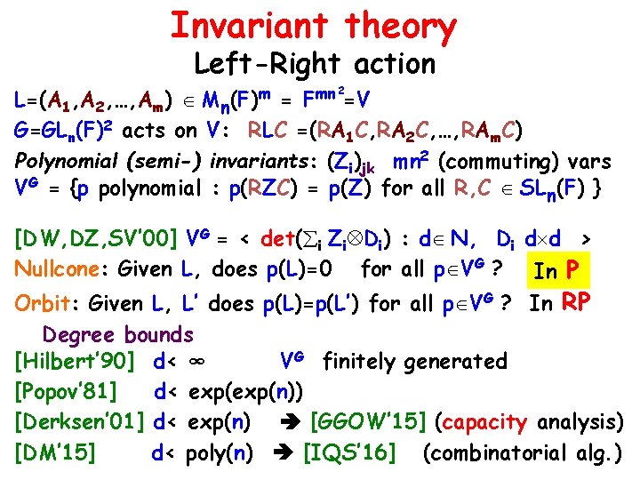
Invariant theory Left-Right action L=(A 1, A 2, …, Am) Mn(F)m = Fmn =V G=GLn(F)2 acts on V: RLC =(RA 1 C, RA 2 C, …, RAm. C) Polynomial (semi-) invariants: (Zi)jk mn 2 (commuting) vars VG = {p polynomial : p(RZC) = p(Z) for all R, C SLn(F) } 2 [DW, DZ, SV’ 00] VG = < det( i Zi Di) : d N, Di d d > Nullcone: Given L, does p(L)=0 for all p VG ? In P Orbit: Given L, L’ does p(L)=p(L’) for all p VG ? In RP Degree bounds [Hilbert’ 90] d< ∞ VG finitely generated [Popov’ 81] d< exp(n)) [Derksen’ 01] d< exp(n) [GGOW’ 15] (capacity analysis) [DM’ 15] d< poly(n) [IQS’ 16] (combinatorial alg. )

Quantum information theory Completely positive maps [Gurvits ’ 04] L=(A 1, A 2, …, Am) Ai Mn(C) completely positive map: Quantum L(P)= i. Ai. PAit (P psd L(P) psd) (noise) operator “Hall Condition” L rank-decreasing if exists P psd s. t. rk(L(P)) < rk(P) [Cohn’ 71] L rank-decreasing L NC-singular. In P Quasi. L doubly stochastic if i. Ait=I i. Ait. Ai=I convex Capacity(L) = inf { det(L(P)) / det(P) : P psd } [Gurvits] L rank-decreasing Cap(L) = 0 L doubly stochastic Cap(L) = 1 L’ = RLC Cap(L’) = Cap(L) det(R)2 det(C)2 Capacity tensorizes: Cap(A 1 D 1, …, Am Dm)=… [GGOW’ 15] Use degree bounds in capacity analysis

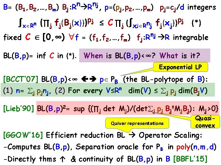
Analysis (and beyond!) Brascamp-Lieb Inequalities [BL’ 76, Lieb’ 90] B = (B 1, B 2, …, Bm) Bj: Rn Rnj p = (pj, p 2, …, pm) pj ≥ 0 ∫x Rn (∏j fj(Bj(x)))pj (B, p): BL data ≤ C ∏j (∫xj Rnj fj(xj))pj fixed C [0, ∞) f = (f 1, f 2, …, fm) fj: Rnj R+ integrable Cauchy-Schwarz, Holder Precopa-Leindler Loomis-Whitney Nelson Hypercontractive Young’s convolution Brunn-Minkowski Lieb’s Non-commutative BL quantitative Helly Bennett-Nez Nonlinear BL Barthe Reverse BL Multilinear estimates, decoupling, Kakeya, restriction, Weyl sums, maximal functions, …

B= (B 1, B 2, …, Bm) Bj: Rn Rnj, p=(pj, p 2, …, pm) pj=cj/d integers ∫x Rn (∏j fj(Bj(x)))pj ≤ C ∏j (∫xj Rnj fj(xj))pj (*) fixed C [0, ∞) f = (f 1, f 2, …, fm) fj: Rnj R integrable BL(B, p)= inf C in (*). When is BL(B, p)<∞? What is it? Exponential LP [BCCT’ 07] BL(B, p)<∞ p PB (the BL-polytope of B): (1) n= j pjnj, (2) For every V≤Rn dim(V) ≤ j pj dim(Bj. V) [Lieb’ 90] BL(B, p)2= sup {(∏j det Mj)/(det j pj Bjt. Mj. Bj): Mj>0} Quiver representations Quasiconvex [GGOW’ 16] Efficient reduction BL Operator Scaling: -Computes BL(B, p), Separation oracle for PB in poly(n, m, d) -Directly thms ↑ & continuity of BL(B, p) in B [BBFL’ 15]

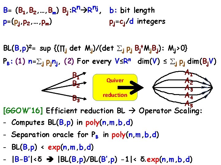
B= (B 1, B 2, …, Bm) Bj: Rn Rnj, b: bit length p=(pj, p 2, …, pm) pj=cj/d integers BL(B, p)2= sup {(∏j det Mj)/(det j pj Bjt. Mj. Bj): Mj>0} PB: (1) n= j pjnj, (2) For every V≤Rn dim(V) ≤ j pj dim(Bj. V) A 1 B 1 Quiver A 2 B 2 A 3 reduction A 4 B 3 A 5 [GGOW’ 16] Efficient reduction BL Operator Scaling: - Computes BL(B, p) in poly(n, m, b, d) - Separation oracle for PB in poly(n, m, b, d) - BL(B, p) < exp(n, m, b, d) - |B-B’|<δ |BL(B, p)/BL(B’, p) -1|< δ. exp(n, m, b, d)

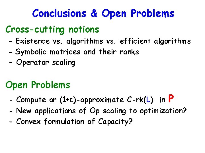
Conclusions & Open Problems Cross-cutting notions - Existence vs. algorithms vs. efficient algorithms - Symbolic matrices and their ranks - Operator scaling Open Problems - Compute or (1+ε)-approximate C-rk(L) in P - New applications of Op scaling to optimization? - Convex formulation of Capacity?