Managing Process Constraints Chapter 5 Copyright 2016 Pearson

Managing Process Constraints Chapter 5 Copyright © 2016 Pearson Education, Limited. 5 -

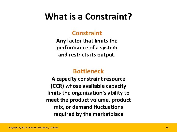
What is a Constraint? Constraint Any factor that limits the performance of a system and restricts its output. Bottleneck A capacity constraint resource (CCR) whose available capacity limits the organization’s ability to meet the product volume, product mix, or demand fluctuations required by the marketplace Copyright © 2016 Pearson Education, Limited. 5 -2

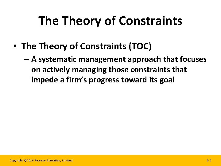
The Theory of Constraints • Theory of Constraints (TOC) – A systematic management approach that focuses on actively managing those constraints that impede a firm’s progress toward its goal Copyright © 2016 Pearson Education, Limited. 5 -3

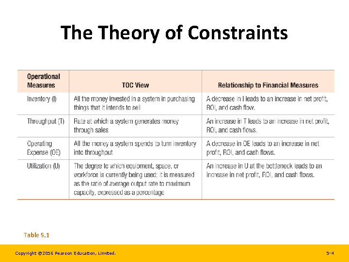
The Theory of Constraints Table 5. 1 Copyright © 2016 Pearson Education, Limited. 5 -4

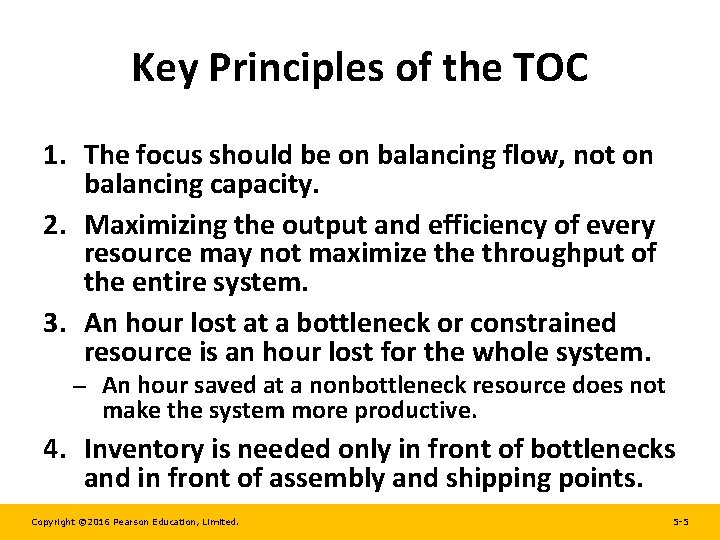
Key Principles of the TOC 1. The focus should be on balancing flow, not on balancing capacity. 2. Maximizing the output and efficiency of every resource may not maximize throughput of the entire system. 3. An hour lost at a bottleneck or constrained resource is an hour lost for the whole system. An hour saved at a nonbottleneck resource does not make the system more productive. 4. Inventory is needed only in front of bottlenecks and in front of assembly and shipping points. Copyright © 2016 Pearson Education, Limited. 5 -5

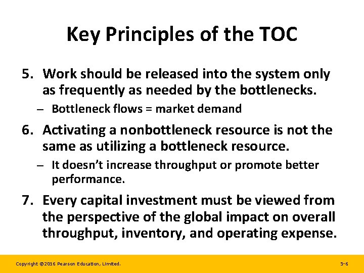
Key Principles of the TOC 5. Work should be released into the system only as frequently as needed by the bottlenecks. Bottleneck flows = market demand 6. Activating a nonbottleneck resource is not the same as utilizing a bottleneck resource. It doesn’t increase throughput or promote better performance. 7. Every capital investment must be viewed from the perspective of the global impact on overall throughput, inventory, and operating expense. Copyright © 2016 Pearson Education, Limited. 5 -6

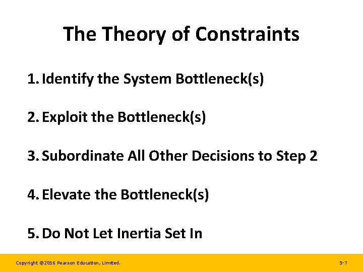
The Theory of Constraints 1. Identify the System Bottleneck(s) 2. Exploit the Bottleneck(s) 3. Subordinate All Other Decisions to Step 2 4. Elevate the Bottleneck(s) 5. Do Not Let Inertia Set In Copyright © 2016 Pearson Education, Limited. 5 -7

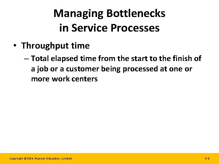
Managing Bottlenecks in Service Processes • Throughput time – Total elapsed time from the start to the finish of a job or a customer being processed at one or more work centers Copyright © 2016 Pearson Education, Limited. 5 -8

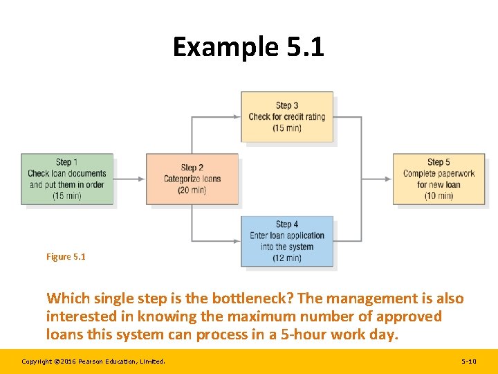
Example 5. 1 • Managers at the First Community Bank are attempting to shorten the time it takes customers with approved loan applications to get their paperwork processed. The flowchart for this process is shown in the next slide. • Approved loan applications first arrive at activity or step 1, where they are checked for completeness and put in order. • At step 2, the loans are categorized into different classes according to the loan amount and whether they are being requested for personal or commercial reasons. • While credit checking commences at step 3, loan application data are entered in parallel into the information system for recordkeeping purposes at step 4. • Finally, all paperwork for setting up the new loan is finished at step 5. The time taken in minutes is given in parentheses. Copyright © 2016 Pearson Education, Limited. 5 -9

Example 5. 1 Figure 5. 1 Which single step is the bottleneck? The management is also interested in knowing the maximum number of approved loans this system can process in a 5 -hour work day. Copyright © 2016 Pearson Education, Limited. 5 -10

Example 5. 1 • We define the bottleneck as step 2, which has the highest time per loan processed. • The throughput time to complete an approved loan application is 15 + 20 + max(15, 12) + 10 = 60 minutes. • The actual time taken for completing an approved loan will be longer than 60 minutes due to nonuniform arrival of applications, variations in actual processing times, and the related factors. • The capacity for loan completions is derived by translating the “minutes per customer” at the bottleneck step to “customer per hour. ” At First Community Bank, it is 3 customers per hour because the bottleneck step 2 can process only 1 customer every 20 minutes (60/3). Copyright © 2016 Pearson Education, Limited. 5 -11

Example 5. 1 • Step 2 is the bottleneck constraint. • The bank will be able to complete a maximum of only three loan accounts per hour, or 15 new loan accounts, in a 5 -hour day. • Management can increase the flow of loan applications by increasing the capacity of Step 2 up to the point where another step becomes the bottleneck. Copyright © 2016 Pearson Education, Limited. 5 -12

Managing Bottlenecks in Manufacturing Processes • Identifying Bottlenecks – Setup times and their associated costs affect the size of the lots traveling through the job or batch processes. Copyright © 2016 Pearson Education, Limited. 5 -13

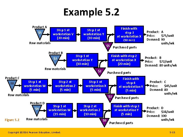
Example 5. 2 Diablo Electronics manufactures four unique products (A, B, C, and D) that are fabricated and assembled in five different workstations (V, W, X, Y, and Z) using a small batch process. Each workstation is staffed by a worker who is dedicated to work a single shift per day at an assigned workstation. Batch setup times have been reduced to such an extent that they can be considered negligible. Figure 5. 2 is a flowchart of the manufacturing process. Diablo can make and sell up to the limit of its demand per week, and no penalties are incurred for not being able to meet all the demand. Which of the five workstations (V, W, X, Y, or Z) has the highest utilization, and thus serves as the bottleneck for Diablo Electronics? Copyright © 2016 Pearson Education, Limited. 5 -14

Example 5. 2 Product A Step 1 at workstation V (30 min) $5 Raw materials $3 Step 1 at workstation Y (10 min) Raw materials $2 Step 1 at workstation W (5 min) (10 min) $5 Purchased parts Product B Product C Finish with step 3 at workstation X Step 2 at workstation Y (10 min) Step 2 at workstation Z (5 min) Finish with step 2 at workstation X (20 min) $2 Step 3 at workstation X (5 min) Figure 5. 2 Finish with step 4 at workstation Y (5 min) $3 Purchased parts $4 Step 1 at workstation W (15 min) Raw materials Copyright © 2016 Pearson Education, Limited. Product: B Price: $72/unit Demand: 80 units/wk Purchased parts Raw materials Product D Product: A Price: $75/unit Demand: 60 units/wk Step 2 at workstation Z (10 min) Finish with step 3 at workstation Y (5 min) $6 Purchased parts Product: C Price: $45/unit Demand: 80 units/wk Product: D Price: $38/unit Demand: 100 units/wk 5 -15

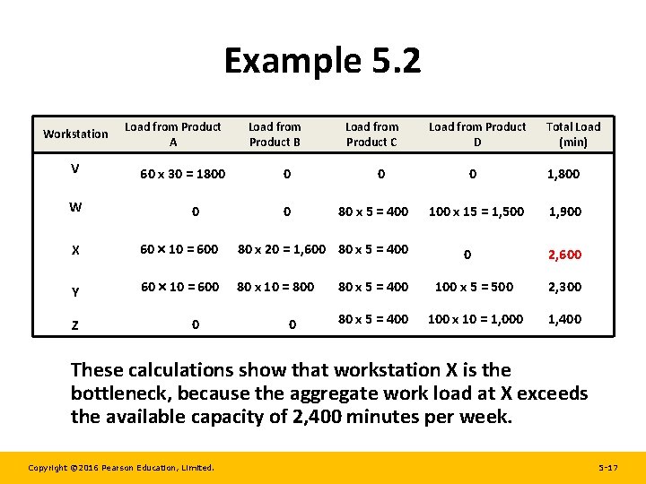
Example 5. 2 • Identify the bottleneck by computing aggregate workloads at each workstation. • The firm wants to satisfy as much of the product demand in a week as it can. • Each week consists of 2, 400 minutes of available production time. • Multiplying the processing time at each station for a given product with the number of units demanded per week yields the workload represented by that product. • These loads are summed across all products going through a workstation to arrive at the total load for the workstation, which is then compared with the others and the existing capacity of 2, 400 minutes. Copyright © 2016 Pearson Education, Limited. 5 -16

Example 5. 2 Workstation V W Load from Product A 60 x 30 = 1800 0 Load from Product B 0 0 Load from Product C 0 80 x 5 = 400 X 60 10 = 600 80 x 20 = 1, 600 80 x 5 = 400 Y 60 10 = 600 80 x 10 = 800 Z 0 0 Load from Product D Total Load (min) 0 1, 800 100 x 15 = 1, 500 1, 900 0 2, 600 80 x 5 = 400 100 x 5 = 500 2, 300 80 x 5 = 400 100 x 10 = 1, 000 1, 400 These calculations show that workstation X is the bottleneck, because the aggregate work load at X exceeds the available capacity of 2, 400 minutes per week. Copyright © 2016 Pearson Education, Limited. 5 -17

Drum-Buffer-Rope Systems Drum-Buffer-Rope A planning and control system that regulates the flow of work-inprocess materials at the bottleneck or the capacity constrained resource (CCR) in a productive system Copyright © 2016 Pearson Education, Limited. 5 -18

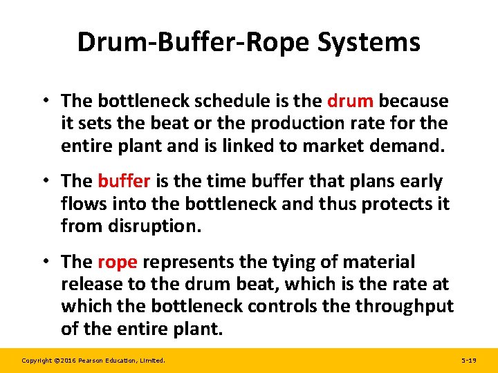
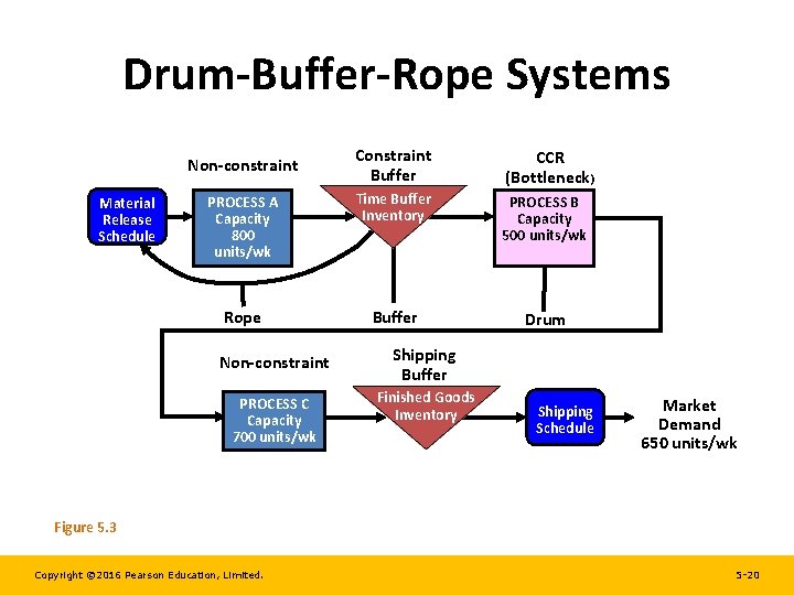
Drum-Buffer-Rope Systems • The bottleneck schedule is the drum because it sets the beat or the production rate for the entire plant and is linked to market demand. • The buffer is the time buffer that plans early flows into the bottleneck and thus protects it from disruption. • The rope represents the tying of material release to the drum beat, which is the rate at which the bottleneck controls the throughput of the entire plant. Copyright © 2016 Pearson Education, Limited. 5 -19

Drum-Buffer-Rope Systems Constraint Buffer CCR (Bottleneck) PROCESS A Capacity 800 units/wk Time Buffer Inventory PROCESS B Capacity 500 units/wk Rope Buffer Drum Non-constraint Material Release Schedule Non-constraint Shipping Buffer PROCESS C Capacity 700 units/wk Finished Goods Inventory Shipping Schedule Market Demand 650 units/wk Figure 5. 3 Copyright © 2016 Pearson Education, Limited. 5 -20

Applying the Theory of Constraints to Product Mix Decisions • Contribution margin – The amount each product contributes to profits and overhead; no fixed costs are considered when making the product mix decision Copyright © 2016 Pearson Education, Limited. 5 -21

Example 5. 3 The senior management at Diablo Electronics (see Example 5. 2) wants to improve profitability by accepting the right set of orders. They collected the following financial data: • Variable overhead costs are $8, 500 per week. • Each worker is paid $18 per hour and is paid for an entire week, regardless of how much the worker is used. • Labor costs are fixed expenses. • The plant operates one 8 -hour shift per day, or 40 hours each week. Currently, decisions are made using the traditional method, which is to accept as much of the highest contribution margin product as possible (up to the limit of its demand), followed by the next highest contribution margin product, and so on until no more capacity is available. Copyright © 2016 Pearson Education, Limited. 5 -22

Example 5. 3 Pedro Rodriguez, the newly hired production supervisor, is knowledgeable about the Theory of Constraints and bottleneck-based scheduling. He believes that profitability can indeed be improved if bottleneck resources were exploited to determine the product mix. What is the change in profits if, instead of the traditional method used by Diablo Electronics, the bottleneck method advocated by Pedro is used to select the product mix? Copyright © 2016 Pearson Education, Limited. 5 -23

Example 5. 3 Decision Rule 1: Traditional Method Step 1: Calculate the contribution margin per unit of each product as shown here. A B C D Price $75. 00 $72. 00 $45. 00 $38. 00 Raw material and purchased parts – 10. 00 – 5. 00 – 10. 00 = Contribution margin $65. 00 $67. 00 $40. 00 $28. 00 When ordered from highest to lowest, the contribution margin per unit sequence of these products is B, A, C, D. Copyright © 2016 Pearson Education, Limited. 5 -24

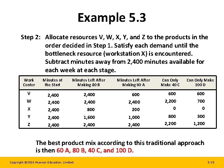
Example 5. 3 Step 2: Allocate resources V, W, X, Y, and Z to the products in the order decided in Step 1. Satisfy each demand until the bottleneck resource (workstation X) is encountered. Subtract minutes away from 2, 400 minutes available for each week at each stage. Work Center Minutes at the Start Minutes Left After Making 80 B Minutes Left After Making 60 A Can Only Make 40 C Can Only Make 100 D V 2, 400 2, 400 800 600 2, 400 200 600 2, 200 0 600 700 0 2, 400 1, 600 2, 400 1, 000 2, 400 800 2, 200 300 1, 200 W X Y Z The best product mix according to this traditional approach is then 60 A, 80 B, 40 C, and 100 D. Copyright © 2016 Pearson Education, Limited. 5 -25

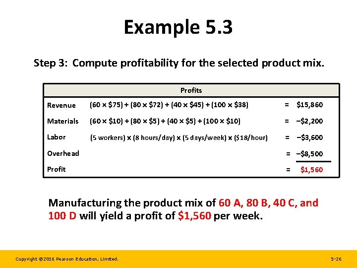
Example 5. 3 Step 3: Compute profitability for the selected product mix. Profits Revenue (60 $75) + (80 $72) + (40 $45) + (100 $38) = $15, 860 Materials (60 $10) + (80 $5) + (40 $5) + (100 $10) = –$2, 200 Labor (5 workers) (8 hours/day) (5 days/week) ($18/hour) = –$3, 600 Overhead = –$8, 500 Profit = $1, 560 Manufacturing the product mix of 60 A, 80 B, 40 C, and 100 D will yield a profit of $1, 560 per week. Copyright © 2016 Pearson Education, Limited. 5 -26

Example 5. 3 Decision Rule 2: Bottleneck Method Select the best product mix according to the dollar contribution margin per minute of processing time at the bottleneck workstation X. This method would take advantage of the principles outlined in the Theory of Constraints and get the most dollar benefit from the bottleneck. Copyright © 2016 Pearson Education, Limited. 5 -27

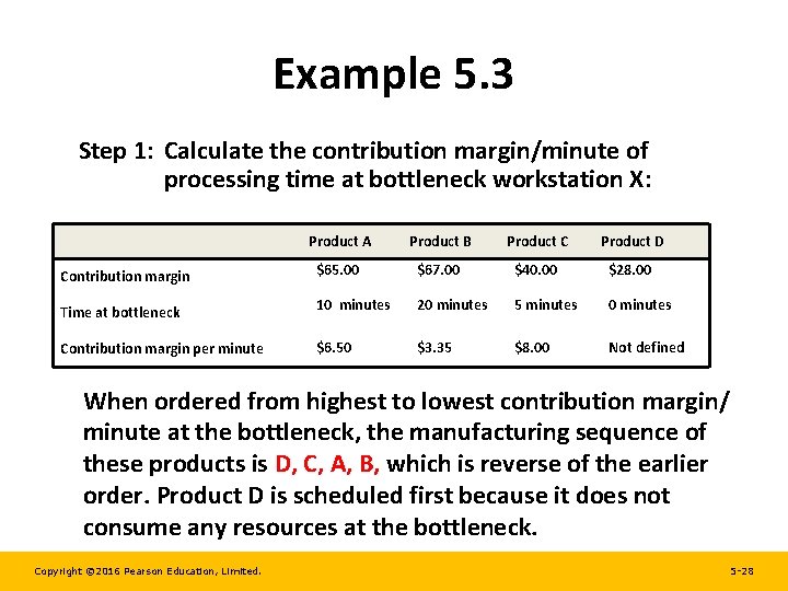
Example 5. 3 Step 1: Calculate the contribution margin/minute of processing time at bottleneck workstation X: Contribution margin Time at bottleneck Contribution margin per minute Product A Product B Product C Product D $65. 00 $67. 00 $40. 00 $28. 00 10 minutes 20 minutes 5 minutes 0 minutes $6. 50 $3. 35 $8. 00 Not defined When ordered from highest to lowest contribution margin/ minute at the bottleneck, the manufacturing sequence of these products is D, C, A, B, which is reverse of the earlier order. Product D is scheduled first because it does not consume any resources at the bottleneck. Copyright © 2016 Pearson Education, Limited. 5 -28

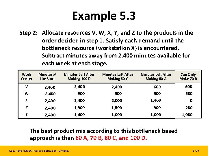
Example 5. 3 Step 2: Allocate resources V, W, X, Y, and Z to the products in the order decided in step 1. Satisfy each demand until the bottleneck resource (workstation X) is encountered. Subtract minutes away from 2, 400 minutes available for each week at each stage. Work Center V W X Y Z Minutes at the Start Minutes Left After Making 100 D Minutes Left After Making 80 C Minutes Left After Making 60 A Can Only Make 70 B 600 500 0 200 1, 000 2, 400 900 2, 400 500 2, 000 600 500 1, 400 2, 400 1, 900 1, 400 1, 500 1, 000 900 1, 000 The best product mix according to this bottleneck based approach is then 60 A, 70 B, 80 C, and 100 D. Copyright © 2016 Pearson Education, Limited. 5 -29

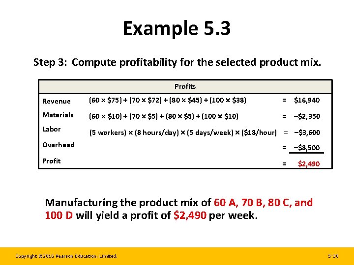
Example 5. 3 Step 3: Compute profitability for the selected product mix. Profits Revenue (60 $75) + (70 $72) + (80 $45) + (100 $38) = $16, 940 Materials (60 $10) + (70 $5) + (80 $5) + (100 $10) = –$2, 350 Labor (5 workers) (8 hours/day) (5 days/week) ($18/hour) = –$3, 600 Overhead = –$8, 500 Profit = $2, 490 Manufacturing the product mix of 60 A, 70 B, 80 C, and 100 D will yield a profit of $2, 490 per week. Copyright © 2016 Pearson Education, Limited. 5 -30

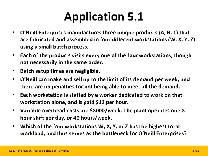
Application 5. 1 • O’Neill Enterprises manufactures three unique products (A, B, C) that are fabricated and assembled in four different workstations (W, X, Y, Z) using a small batch process. • Each of the products visits every one of the four workstations, though not necessarily in the same order. • Batch setup times are negligible. • O’Neill can make and sell up to the limit of its demand per week, and there are no penalties for not being able to meet all the demand. • Each workstation is staffed by a worker dedicated to work on that workstation alone, and is paid $12 per hour. • Variable overhead costs are $8000/week. The plant operates one 8 hour shift per day, or 40 hours/week. • Which of the four workstations W, X, Y, or Z has the highest total workload, and thus serves as the bottleneck for O’Neill Enterprises? Copyright © 2016 Pearson Education, Limited. 5 -31

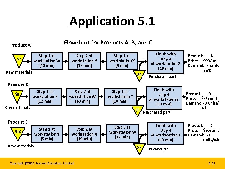
Application 5. 1 Flowchart for Products A, B, and C Product A $7 Step 1 at workstation W (10 min) Step 2 at workstation Y (15 min) Finish with step 4 at workstation Z (16 min) Step 3 at workstation X (9 min) Raw materials $6 Product B $9 Step 1 at workstation X (12 min) Step 2 at workstation W (10 min) Raw materials $5 Purchased part Product C $10 Purchased part Finish with step 4 at workstation Z (13 min) Step 3 at workstation Y (10 min) Step 1 at workstation Y (5 min) Step 2 at workstation X (10 min) Raw materials Copyright © 2016 Pearson Education, Limited. Finish with step 4 at workstation Z (10 min) Step 3 at workstation W (12 min) $5 Product: A Price: $90/unit Demand: 65 units /wk Product: B Price: $85/unit Demand: 70 units/ wk Product: C Price: $80/unit Demand: 80 units/wk Purchased part 5 -32

Application 5. 1 Identify the bottleneck by computing total workload at each workstation. The firm wants to satisfy as much of the product demand in a week as it can. Each week consists of 2400 minutes of available production time. Multiplying the processing time at each station for a given product with the number of units demanded per week yields the capacity load. These loads are summed across all products going through that workstation and then compared with the existing capacity of 2400 minutes. Copyright © 2016 Pearson Education, Limited. 5 -33

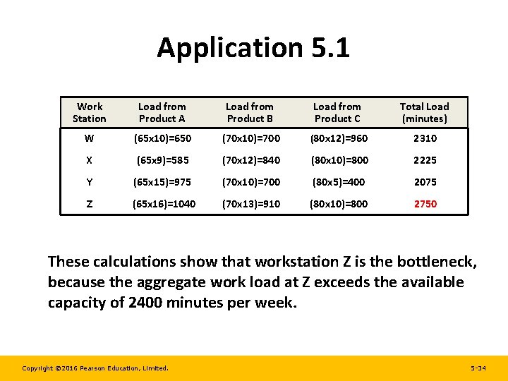
Application 5. 1 Work Station Load from Product A Load from Product B Load from Product C Total Load (minutes) W (65 x 10)=650 (70 x 10)=700 (80 x 12)=960 2310 X (65 x 9)=585 (70 x 12)=840 (80 x 10)=800 2225 Y (65 x 15)=975 (70 x 10)=700 (80 x 5)=400 2075 Z (65 x 16)=1040 (70 x 13)=910 (80 x 10)=800 2750 These calculations show that workstation Z is the bottleneck, because the aggregate work load at Z exceeds the available capacity of 2400 minutes per week. Copyright © 2016 Pearson Education, Limited. 5 -34

Application 5. 2 • The senior management at O’Neill wants to improve the profitability of the firm by accepting the right set of orders. • Currently, decisions are made to accept as much of the highest contribution margin product as possible (up to the limit of its demand), followed by the next highest contribution margin product, and so on until no more capacity is available. • Since the firm cannot satisfy all the demand, the product mix must be chosen carefully. • Jane Hathaway, the newly hired production supervisor, is knowledgeable about the Theory of Constraints and bottleneck based scheduling. She believes that profitability can indeed be approved if bottleneck resources were exploited to determine the product mix. Copyright © 2016 Pearson Education, Limited. 5 -35

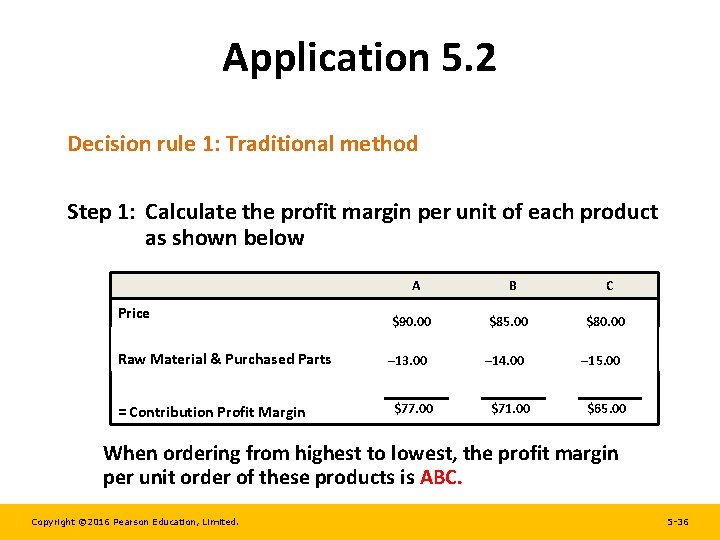
Application 5. 2 Decision rule 1: Traditional method Step 1: Calculate the profit margin per unit of each product as shown below Price Raw Material & Purchased Parts = Contribution Profit Margin A B C $90. 00 $85. 00 $80. 00 – 13. 00 – 14. 00 – 15. 00 $77. 00 $71. 00 $65. 00 When ordering from highest to lowest, the profit margin per unit order of these products is ABC. Copyright © 2016 Pearson Education, Limited. 5 -36

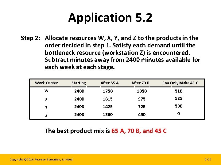
Application 5. 2 Step 2: Allocate resources W, X, Y, and Z to the products in the order decided in step 1. Satisfy each demand until the bottleneck resource (workstation Z) is encountered. Subtract minutes away from 2400 minutes available for each week at each stage. Work Center Starting After 65 A After 70 B Can Only Make 45 C W 2400 1750 1050 510 X 2400 1815 975 525 Y 2400 1425 725 500 Z 2400 1360 450 0 The best product mix is 65 A, 70 B, and 45 C Copyright © 2016 Pearson Education, Limited. 5 -37

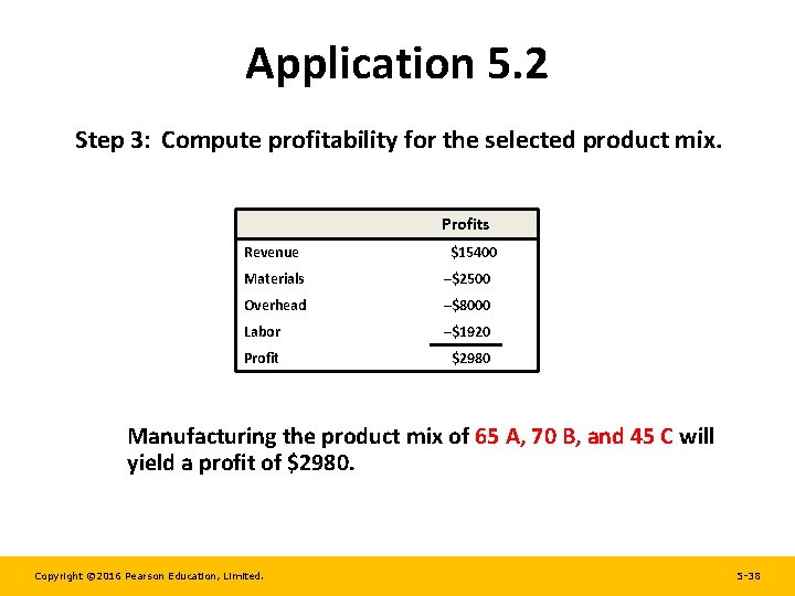
Application 5. 2 Step 3: Compute profitability for the selected product mix. Revenue Profits $15400 Materials –$2500 Overhead –$8000 Labor –$1920 Profit $2980 Manufacturing the product mix of 65 A, 70 B, and 45 C will yield a profit of $2980. Copyright © 2016 Pearson Education, Limited. 5 -38

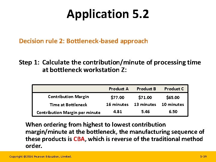
Application 5. 2 Decision rule 2: Bottleneck-based approach Step 1: Calculate the contribution/minute of processing time at bottleneck workstation Z: Product A Product B Product C Time at Bottleneck $77. 00 16 minutes $71. 00 13 minutes $65. 00 10 minutes Contribution Margin per minute 4. 81 5. 46 6. 50 Contribution Margin When ordering from highest to lowest contribution margin/minute at the bottleneck, the manufacturing sequence of these products is CBA, which is reverse of the traditional method order. Copyright © 2016 Pearson Education, Limited. 5 -39

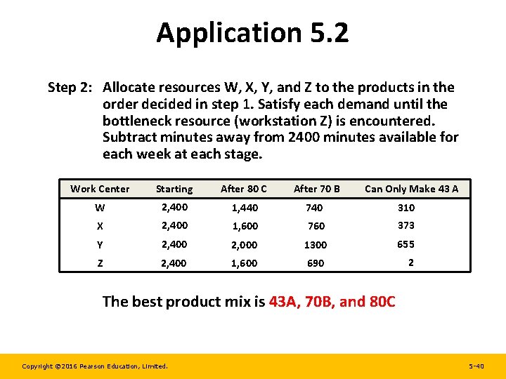
Application 5. 2 Step 2: Allocate resources W, X, Y, and Z to the products in the order decided in step 1. Satisfy each demand until the bottleneck resource (workstation Z) is encountered. Subtract minutes away from 2400 minutes available for each week at each stage. Work Center Starting After 80 C After 70 B Can Only Make 43 A W 2, 400 1, 440 740 310 X 2, 400 1, 600 760 373 Y 2, 400 2, 000 1300 655 Z 2, 400 1, 600 690 2 The best product mix is 43 A, 70 B, and 80 C Copyright © 2016 Pearson Education, Limited. 5 -40

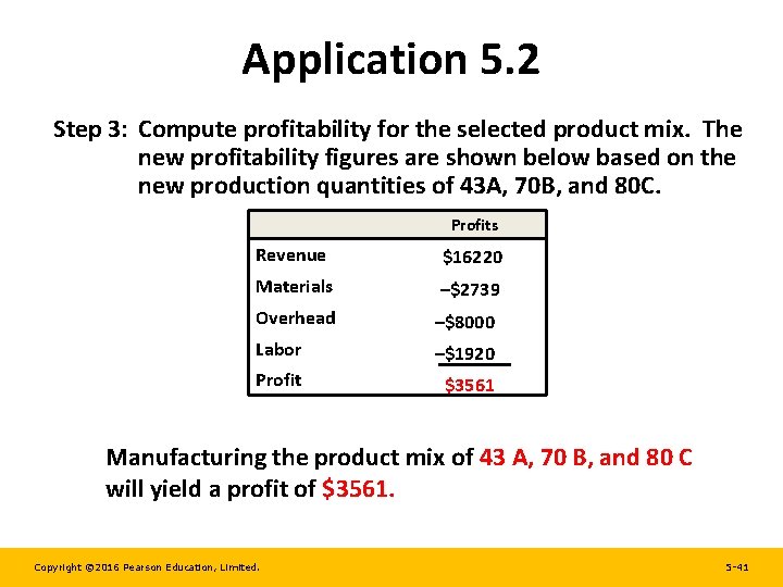
Application 5. 2 Step 3: Compute profitability for the selected product mix. The new profitability figures are shown below based on the new production quantities of 43 A, 70 B, and 80 C. Profits Revenue $16220 Materials –$2739 Overhead –$8000 Labor –$1920 Profit $3561 Manufacturing the product mix of 43 A, 70 B, and 80 C will yield a profit of $3561. Copyright © 2016 Pearson Education, Limited. 5 -41

Managing Constraints in a Line Process • Line Balancing – The assignment of work to stations in a line so as to achieve the desired output rate with the smallest number of workstations • Precedence Diagram – A diagram that allows one to visualize immediate predecessors better Copyright © 2016 Pearson Education, Limited. 5 -42

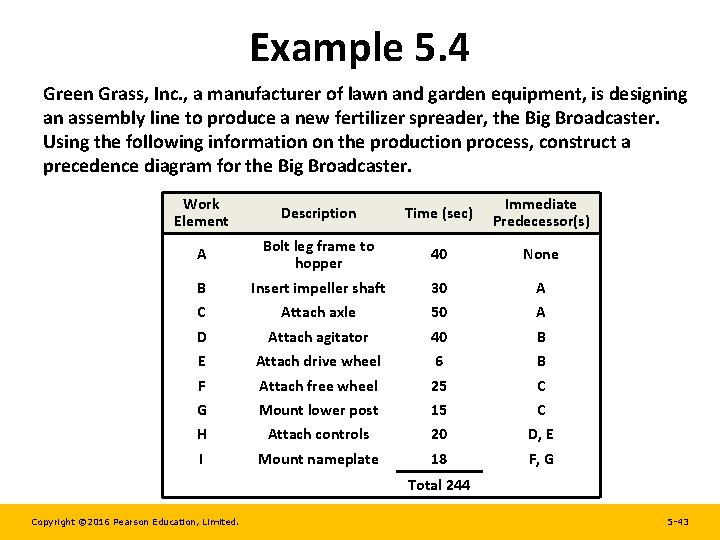
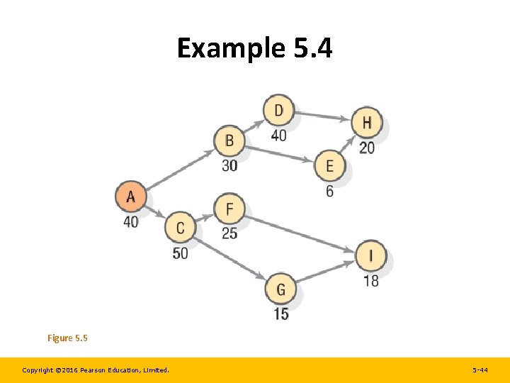
Example 5. 4 Green Grass, Inc. , a manufacturer of lawn and garden equipment, is designing an assembly line to produce a new fertilizer spreader, the Big Broadcaster. Using the following information on the production process, construct a precedence diagram for the Big Broadcaster. Work Element Description Time (sec) Immediate Predecessor(s) A Bolt leg frame to hopper 40 None B Insert impeller shaft 30 A C Attach axle 50 A D Attach agitator 40 B E Attach drive wheel 6 B F Attach free wheel 25 C G Mount lower post 15 C H Attach controls 20 D, E I Mount nameplate 18 F, G Total 244 Copyright © 2016 Pearson Education, Limited. 5 -43

Example 5. 4 Figure 5. 5 Copyright © 2016 Pearson Education, Limited. 5 -44

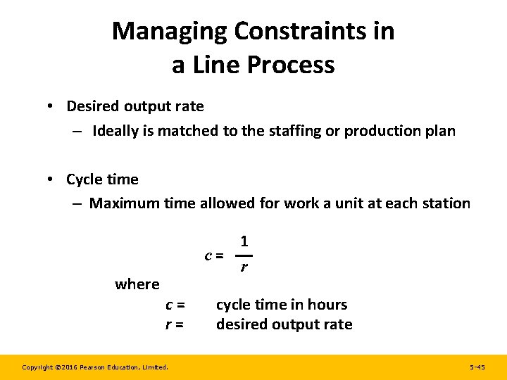
Managing Constraints in a Line Process • Desired output rate – Ideally is matched to the staffing or production plan • Cycle time – Maximum time allowed for work a unit at each station where 1 c = r = Copyright © 2016 Pearson Education, Limited. cycle time in hours desired output rate 5 -45

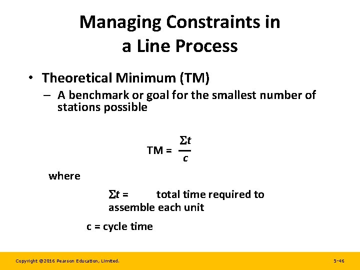
Managing Constraints in a Line Process • Theoretical Minimum (TM) – A benchmark or goal for the smallest number of stations possible t TM = c where t = total time required to assemble each unit c = cycle time Copyright © 2016 Pearson Education, Limited. 5 -46

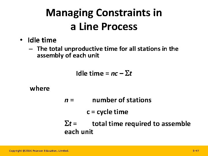
Managing Constraints in a Line Process • Idle time – The total unproductive time for all stations in the assembly of each unit Idle time = nc – t where n = number of stations c = cycle time t = total time required to assemble each unit Copyright © 2016 Pearson Education, Limited. 5 -47

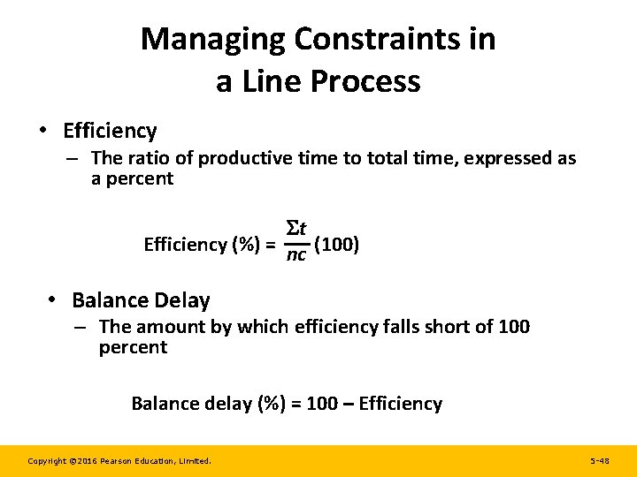
Managing Constraints in a Line Process • Efficiency – The ratio of productive time to total time, expressed as a percent t Efficiency (%) = (100) nc • Balance Delay – The amount by which efficiency falls short of 100 percent Balance delay (%) = 100 – Efficiency Copyright © 2016 Pearson Education, Limited. 5 -48

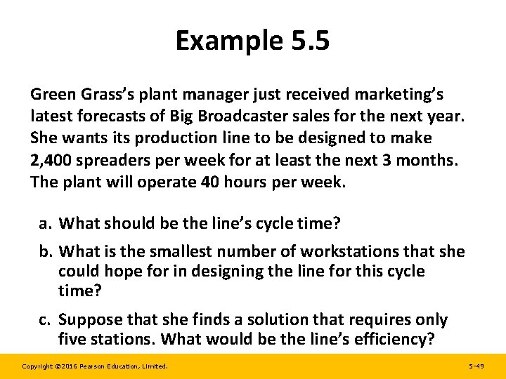
Example 5. 5 Green Grass’s plant manager just received marketing’s latest forecasts of Big Broadcaster sales for the next year. She wants its production line to be designed to make 2, 400 spreaders per week for at least the next 3 months. The plant will operate 40 hours per week. a. What should be the line’s cycle time? b. What is the smallest number of workstations that she could hope for in designing the line for this cycle time? c. Suppose that she finds a solution that requires only five stations. What would be the line’s efficiency? Copyright © 2016 Pearson Education, Limited. 5 -49

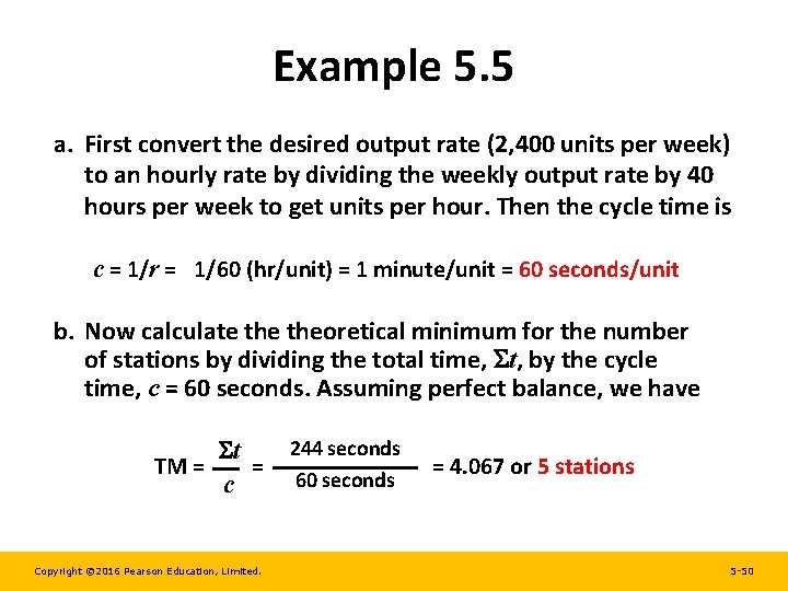
Example 5. 5 a. First convert the desired output rate (2, 400 units per week) to an hourly rate by dividing the weekly output rate by 40 hours per week to get units per hour. Then the cycle time is c = 1/r = 1/60 (hr/unit) = 1 minute/unit = 60 seconds/unit b. Now calculate theoretical minimum for the number of stations by dividing the total time, t, by the cycle time, c = 60 seconds. Assuming perfect balance, we have 244 seconds t = = 4. 067 or 5 stations TM = 60 seconds c Copyright © 2016 Pearson Education, Limited. 5 -50

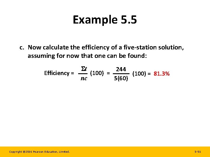
Example 5. 5 c. Now calculate the efficiency of a five-station solution, assuming for now that one can be found: t 244 Efficiency = (100) = 81. 3% nc 5(60) Copyright © 2016 Pearson Education, Limited. 5 -51

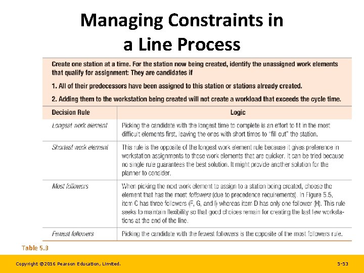
Managing Constraints in a Line Process • Finding a Solution – The goal is to cluster the work elements into workstations so that: • The number of workstations required is minimized • The precedence and cycle-time requirements are not violated Copyright © 2016 Pearson Education, Limited. 5 -52

Managing Constraints in a Line Process Table 5. 3 Copyright © 2016 Pearson Education, Limited. 5 -53

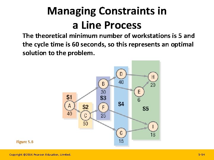
Managing Constraints in a Line Process The theoretical minimum number of workstations is 5 and the cycle time is 60 seconds, so this represents an optimal solution to the problem. Figure 5. 6 Copyright © 2016 Pearson Education, Limited. 5 -54

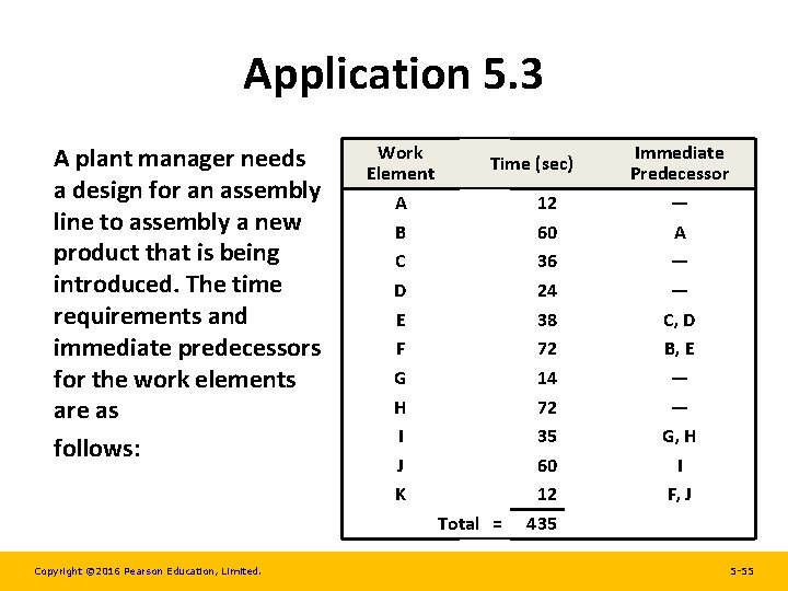
Application 5. 3 A plant manager needs a design for an assembly line to assembly a new product that is being introduced. The time requirements and immediate predecessors for the work elements are as follows: Work Element A B C D E F G H I J K Time (sec) Total = Copyright © 2016 Pearson Education, Limited. 12 60 36 24 38 72 14 72 35 60 12 435 Immediate Predecessor ― A ― ― C, D B, E ― ― G, H I F, J 5 -55

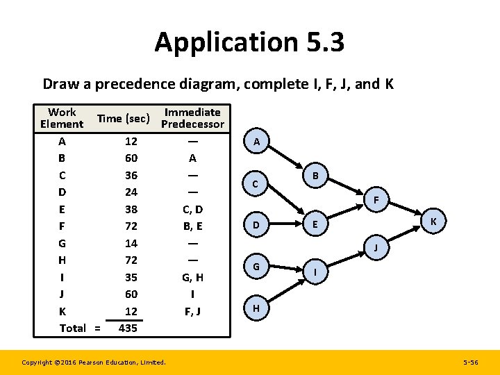
Application 5. 3 Draw a precedence diagram, complete I, F, J, and K Work Time (sec) Immediate Element Predecessor A 12 ― B 60 A C 36 ― D 24 ― E 38 C, D F 72 B, E G 14 ― H 72 ― I 35 G, H J 60 I K 12 F, J Total = 435 Copyright © 2016 Pearson Education, Limited. A C B F D K E J G I H 5 -56

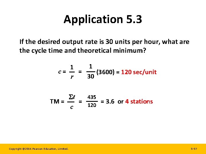
Application 5. 3 If the desired output rate is 30 units per hour, what are the cycle time and theoretical minimum? 1 1 c = = (3600) = 120 sec/unit 30 r 435 t TM = = = 3. 6 or 4 stations 120 c Copyright © 2016 Pearson Education, Limited. 5 -57

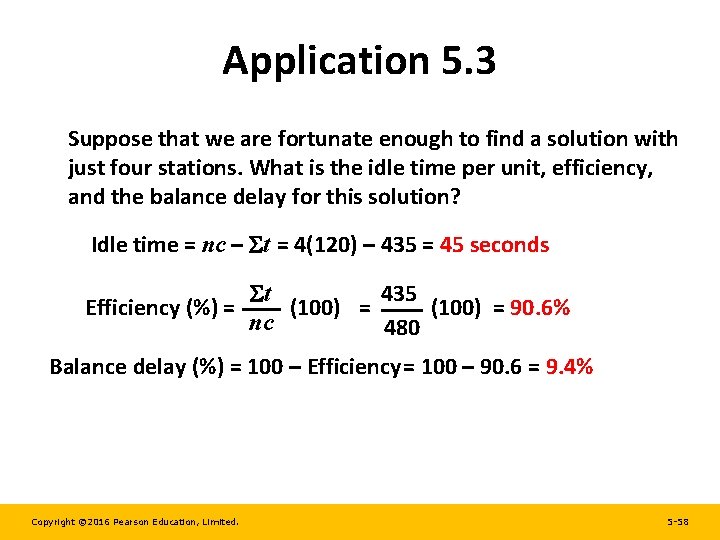
Application 5. 3 Suppose that we are fortunate enough to find a solution with just four stations. What is the idle time per unit, efficiency, and the balance delay for this solution? Idle time = nc – t = 4(120) – 435 = 45 seconds 435 t Efficiency (%) = (100) = 90. 6% nc 480 Balance delay (%) = 100 – Efficiency = 100 – 90. 6 = 9. 4% Copyright © 2016 Pearson Education, Limited. 5 -58

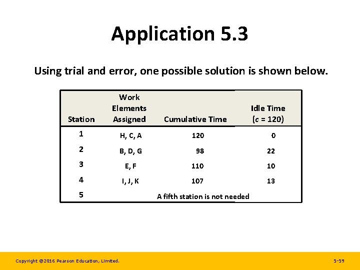
Application 5. 3 Using trial and error, one possible solution is shown below. Station Work Elements Assigned 1 H, C, A 120 0 2 B, D, G 98 22 3 E, F 110 10 4 I, J, K 107 13 5 Copyright © 2016 Pearson Education, Limited. Cumulative Time Idle Time (c = 120) A fifth station is not needed 5 -59

Rebalancing the Assembly Line • Managerial Considerations – Pacing is the movement of product from one station to the next as soon as the cycle time has elapsed – Behavioral factors such as absenteeism, turnover, and grievances can increase after installing production lines. – The number of models produced complicates scheduling and necessitates good communication. – Cycle times are dependent on the desired output rate or sometimes on the maximum workstations allowed. Copyright © 2016 Pearson Education, Limited. 5 -60

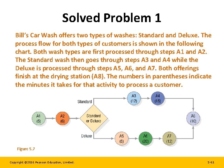
Solved Problem 1 Bill’s Car Wash offers two types of washes: Standard and Deluxe. The process flow for both types of customers is shown in the following chart. Both wash types are first processed through steps A 1 and A 2. The Standard wash then goes through steps A 3 and A 4 while the Deluxe is processed through steps A 5, A 6, and A 7. Both offerings finish at the drying station (A 8). The numbers in parentheses indicate the minutes it takes for that activity to process a customer. Figure 5. 7 Copyright © 2016 Pearson Education, Limited. 5 -61

Solved Problem 1 a. Which step is the bottleneck for the Standard car wash process? For the Deluxe car wash process? b. What is the capacity (measured as customers served per hour) of Bill’s Car Wash to process Standard and Deluxe customers? Assume that no customers are waiting at step A 1, A 2, or A 8. c. If 60 percent of the customers are Standard and 40 percent are Deluxe, what is the average capacity of the car wash in customers per hour? d. Where would you expect Standard wash customers to experience waiting lines, assuming that new customers are always entering the shop and that no Deluxe customers are in the shop? Where would the Deluxe customers have to wait, assuming no Standard customers? Copyright © 2016 Pearson Education, Limited. 5 -62

Solved Problem 1 a. Step A 4 is the bottleneck for the Standard car wash process, and Step A 6 is the bottleneck for the Deluxe car wash process, because these steps take the longest time in the flow. b. The capacity for Standard washes is 4 customers per hour because the bottleneck step A 4 can process 1 customer every 15 minutes (60/15). The capacity for Deluxe car washes is 3 customers per hour (60/20). These capacities are derived by translating the “minutes per customer” of each bottleneck activity to “customers per hour. ” c. The average capacity of the car wash is (0. 60 4) + (0. 40 3) = 3. 6 customers per hour. Copyright © 2016 Pearson Education, Limited. 5 -63

Solved Problem 1 d. Standard wash customers would wait before steps A 1, A 2, A 3, and A 4 because the activities that immediately precede them have a higher rate of output (i. e. , smaller processing times). Deluxe wash customers would experience a wait in front of steps A 1, A 2, and A 6 for the same reasons. A 1 is included for both types of washes because the arrival rate of customers could always exceed the capacity of A 1. Copyright © 2016 Pearson Education, Limited. 5 -64

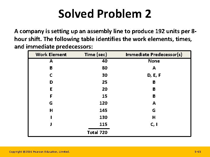
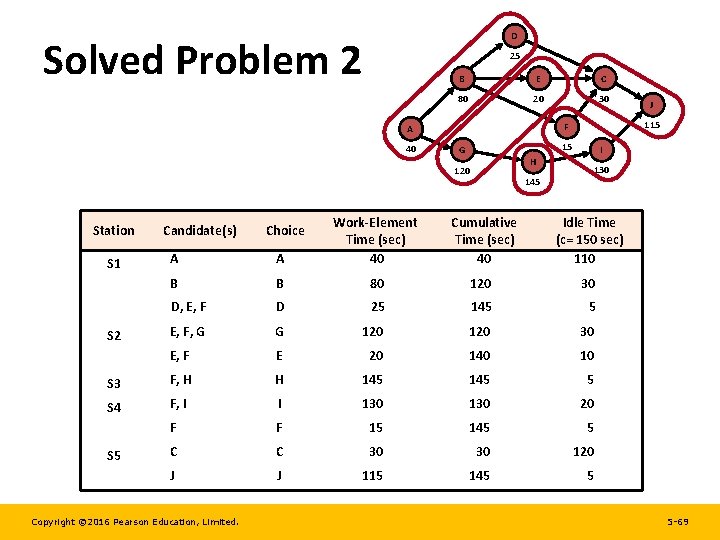
Solved Problem 2 A company is setting up an assembly line to produce 192 units per 8 hour shift. The following table identifies the work elements, times, and immediate predecessors: Work Element A B C D E F G H I J Time (sec) 40 80 30 25 20 15 120 145 130 115 Immediate Predecessor(s) None A D, E, F B B B A G H C, I Total 720 Copyright © 2016 Pearson Education, Limited. 5 -65

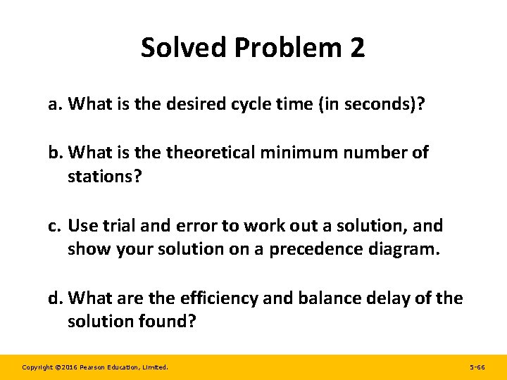
Solved Problem 2 a. What is the desired cycle time (in seconds)? b. What is theoretical minimum number of stations? c. Use trial and error to work out a solution, and show your solution on a precedence diagram. d. What are the efficiency and balance delay of the solution found? Copyright © 2016 Pearson Education, Limited. 5 -66

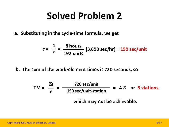
Solved Problem 2 a. Substituting in the cycle-time formula, we get 1 8 hours c = = (3, 600 sec/hr) = 150 sec/unit r 192 units b. The sum of the work-element times is 720 seconds, so 720 sec/unit t TM = = = 4. 8 or 5 stations 150 sec/unit-station c which may not be achievable. Copyright © 2016 Pearson Education, Limited. 5 -67

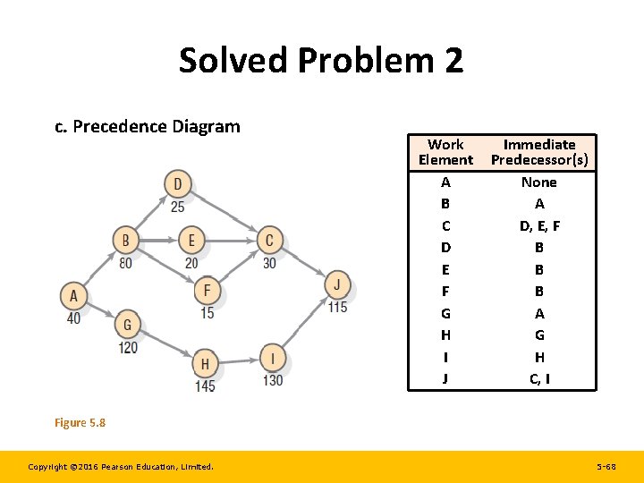
Solved Problem 2 c. Precedence Diagram Work Element A B C D E F G H I J Immediate Predecessor(s) None A D, E, F B B B A G H C, I Figure 5. 8 Copyright © 2016 Pearson Education, Limited. 5 -68

D Solved Problem 2 25 B E C 80 20 30 40 115 F A 15 G H 120 145 130 A A B B 80 120 30 D, E, F D 25 145 5 E, F, G G 120 30 E, F E 20 140 10 S 3 F, H H 145 5 S 4 F, I I 130 20 F F 15 145 5 C C 30 30 120 J J 115 145 5 S 1 S 2 S 5 Candidate(s) Copyright © 2016 Pearson Education, Limited. Choice Cumulative Time (sec) 40 I Work-Element Time (sec) 40 Station J Idle Time (c= 150 sec) 110 5 -69

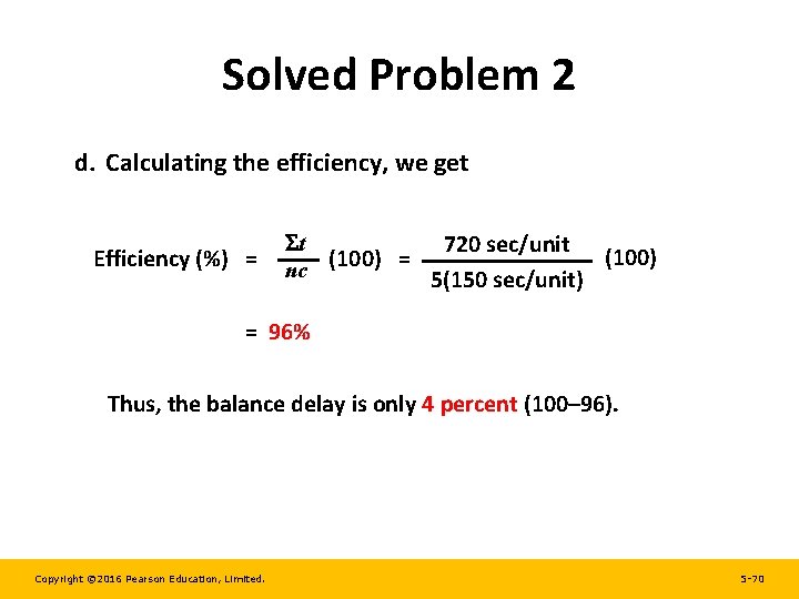
Solved Problem 2 d. Calculating the efficiency, we get t Efficiency (%) = (100) = nc 720 sec/unit (100) 5(150 sec/unit) = 96% Thus, the balance delay is only 4 percent (100– 96). Copyright © 2016 Pearson Education, Limited. 5 -70