Macro stress Testing Credit Risk A Panel Econometric

Macro stress Testing Credit Risk: A Panel Econometric Estimation with Ugandan Data by Charles Augustine Abuka Director, Financial Stability Department BANK OF UGANDA Prepared for the CMI Course on Macro stress testing August 22, 2013 KSMS, Nairobi, Kenya

OUTLINE 2

Outline • • • Applications in modelling the financial sector Introduction to Panel Data Models Practical Applications Using Ugandan Data Further Topics Concluding Remarks 3

APPLICATIONS IN MODELLING SOURCES OF SYSTEMIC RISK IN THE BANKING SECTOR 4

The empirical literature overview Author (s) Methodology and Economies Results Gambera [2000] The authour used bivariate VAR (employing variables such as unemployment, sector income, number of bankrupcies, car sales and agricultural, commercial, industrial and real estate loans) and investigated the impact of economic development on loan portfolio quality for the case of the USA. This study revealed the link between macroeconomics dynamics and banks asset quality, where yields can be used to make accurate predictions of future effects of the business cycle on assets quality and cyclical factors can be used for asset quality forecasting. Arpa et al [2001] The authours used single equation regression analysis, focusing on risk provisions and the operating income of Austrian banks. The authours conclude that the share of risk provisions in the total loans of the banking sector varies indirectly with real GDP and real interest rates and directly with CPI inflation and real estate price inflation. Blaschke and Jones [2001] The authors applied a VAR methodology to investigate the transmission from real GDP, inflation, nominal interest rate and the terms of trade to NPL ratio for the case of the USA. The authours discuss the impact of GDP growth and the business cycle on credit risk and also on the quality of bank loans 5

The empirical literature overview Author (s) Methodology and Economies Results Gropp et al [2002] The authours suggested a comparison of an equitybased indicator (distance to default) and a bond-market related (subordinated debt spread) in emerging market economies. The spreads do contract in line with a positive outlook for economies, corporate bond yield decline, generally maintaining their spreads to government bonds at fairly low levels, amid signs of stable-toimproving credit quality and favourable liquidity conditions. Gerlach et al, [2005] The author relied on regression analysis (for the case of Hong Kong) and employed nominal interest rates, the CPI, property prices, equity prices, and number of bankruptcies, the unemployment rate and real GDP as explanatory variables. The analysis indicates that the NPL ratio rises with increasing nominal interest rates and an increasing number of bankruptcies, but decreases with higher CPI inflation, economic growth, and property price inflation. Deflation squeezes out corporate profitability and adversely affects borrowers ability to pay. Quagliariello [2003] The authour presents a regression between the evolution of NPLs as a dependent variable and a set of explanatory variables for the case of Italy: the real GDP growth rate, the growth of real gross fixed investment and consumption, changes in the unemployment rate, the CPI, the real exchange rate and the M 2 growth rate. The authour concluded that decreasing real GDP growth and increasing unemployment have a significantly adverse effect on loan portfolio quality, while the real exchange rate and consumer price index fail to significantly affect it. 6

The empirical literature overview Author (s) Methodology and Economies Results Popiera [2006] The author explored the relationship between banking sector performance and the quality of regulation and supervision as measured by the Basel Core Principles for Effective Supervision using the panel data for 65 economies. The study revealed the significant positive impact of higher compliance with the Basel Core Principles on banking sector performance as measure by NPL and net interest margin (after controlling for the level of development of the economy and financial system). Manasoo and Mayes [2009] The authours presented a panel logit model for the CEE between the evolution of NPLs and set of explanatory variables: liquidity ratio, inverse liquidity ratio, loan to asset ratio, equity to asset ratio, cost to income ratio and macroeconomic variables. The authours claim that declining GDP growth and the instability of external and internal environments leads to a worsening of banking sector results and financial stability indicators in the CEE. Baboucek and Jankar [2005] The authours investigated economic developments in the Czech banking sector through unemployment, real GDP growth, exports, imports, the real effective exchange rate, the CPI and credit growth as indicators of NPL ratio performance using an unrestricted VAR methodology. The study showed that the appreciation of the real effective exchange rate does not deteriorate the NPL ratio; increasing unemployment and inflation deteriorate the NPL ratio, while faster GDP growth decelerates the NPL ratio. 7

The empirical literature overview Author (s) Methodology and Economies Results Hoggarth et al [2005] The authours applied the VAR approach to investigate the link between loan write-offs and the output gap, retail prices, real estate prices, the nominal short term interest rates and the real exchange rate for the case of the United Kingdom. The important factors indirectly influencing financial stability and loan portfolio quality are the dynamics of inflation and interest rates. Chihak et al [2007] The authours compared system focused stress testing methods (VAR, Monte Carlo Simulations, etc) and discussed issues related to the design of stress tests for the Czech banking system. The authours suggest (besides banking sector indicators such as capital adequacy, credit risk and other relevant factors) incorporating different shocks into models, non bank financial indicators and relevant macroeconomic factors ( e. g. the exchange rate and the interest rate) in order to perform stress testing Babihuga [2007] The authour investigated the relationship between macroeconomic variables and financial stability indictors (like capital adequacy, asset quality and profitability) in the case of the European, Asian and Sub -Saharan Africa economies. The authour presented a regression between the evolution of NPL as a dependent variable and a set of explanatory variables: the quality of banking sector supervision measured by an index of compliance with the Basel Core Principles, terms of trade, unemployment, lending rates, the real effective exchange rate and the business cycle component of GDP. The authour showed that financial stability indicators fluctuate strongly with the business cycle and the inflation rate. ; and that the cycle component of real GDP has a negative relationship with capital adequacy and NPLs. There is also an important degree of heterogeneity across the sample of countries (European, Asian and Sub-Saharan Africa economies) between macroeconomic and financial stability indicators. The relationship between the business cycle and capital adequacy is more ambiguous and it appear to be counter cyclical (except in Asian and Sub Saharan African, where it is procyclical). 8

The empirical literature overview Author (s) Methodology and Economies Results Jakubik [2007] The authour employed the regression method for NPL inflow estimation (in the case of the Czech Republic) using real GDP, real effective exchange rates, the CPI, the loan to GDP ratio, unemployment, and the real interest rate as explanatory variables. The default rate for the corporate sector is determined by the appreciation of the real effective exchange rate and by the increase in the loan to GDP ratio; meanwhile, the default rate for households deteriorates via unemployment and interest-rate increases. Zeman and Jurca [2008] The authors applied the multivariate regression method using real GDP, the output gap, exports, industrial production, oil prices, the CPI, M 1, nominal interest rates, and nominal exchange rates as explanatory variables for NPL dynamics in the case of slovakia. Real GDP, the nominal exchange rate and nominal interest rate are the most important variable influencing NPL dynamics. A slow down in GDP growth is not expected to substantially threaten the banking system. Exposure to interest rate growth through direct channels and foreign currency risk through indirect channels was shown to be due to the high level of openness of the economy. 9

The empirical literature overview Author (s) Methodology and Economies Results Uhde and Heimeshoff [2009] The authours provided empirical evidence in the case of the EU-25, that the national banking market concentration has a negative impact on European Banks’ financial soundness as measured by the Z score technique (while controlling for macroeconomic, bank-specific regulatory and institutional factors. The authours reveal that Eastern European Banking markets exhibit a lower level of competitive pressure, fewer diversification opportunities and a higher fraction of government-owned banks, which are more prone to financial fragility. 10

PANEL DATA REGRESSION MODELS 11

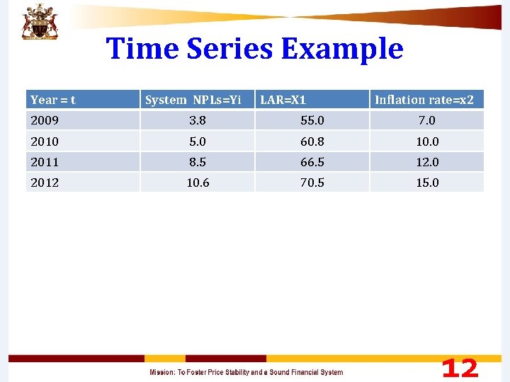
Time Series Example Year = t System NPLs=Yi LAR=X 1 Inflation rate=x 2 2009 3. 8 55. 0 7. 0 2010 5. 0 60. 8 10. 0 2011 8. 5 66. 5 12. 0 2012 10. 6 70. 5 15. 0 12

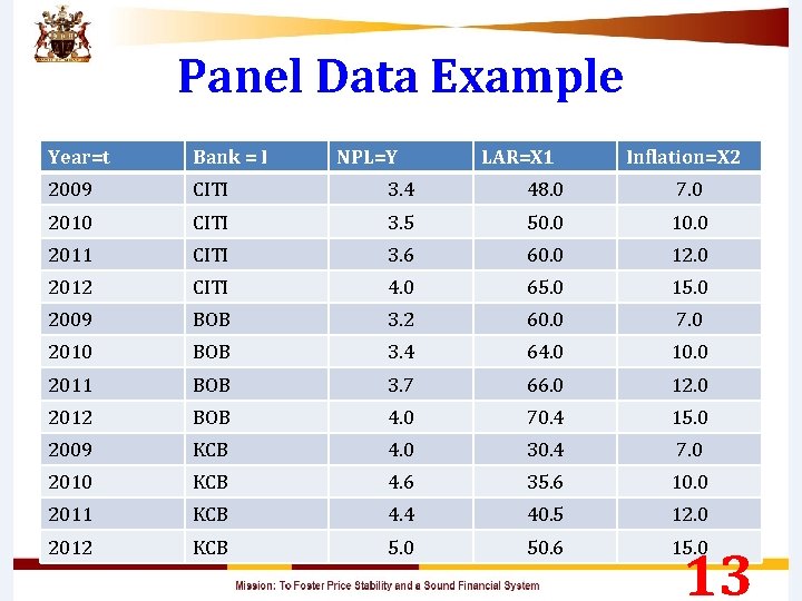
Panel Data Example Year=t Bank = I NPL=Y LAR=X 1 Inflation=X 2 2009 CITI 3. 4 48. 0 7. 0 2010 CITI 3. 5 50. 0 10. 0 2011 CITI 3. 6 60. 0 12. 0 2012 CITI 4. 0 65. 0 15. 0 2009 BOB 3. 2 60. 0 7. 0 2010 BOB 3. 4 64. 0 10. 0 2011 BOB 3. 7 66. 0 12. 0 2012 BOB 4. 0 70. 4 15. 0 2009 KCB 4. 0 30. 4 7. 0 2010 KCB 4. 6 35. 6 10. 0 2011 KCB 4. 4 40. 5 12. 0 2012 KCB 5. 0 50. 6 15. 0 13

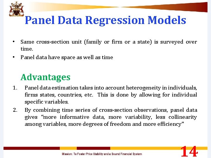
Panel Data Regression Models • Same cross-section unit (family or firm or a state) is surveyed over time. • Panel data have space as well as time Advantages 1. 2. Panel data estimation takes into account heterogeneity in individuals, firms states, countries, etc. This is done by allowing for individual specific variables. By combining time series of cross-section observations, panel data gives “more informative data, more variability, less collinearity among variables, more degrees of freedom and more efficiency” 14

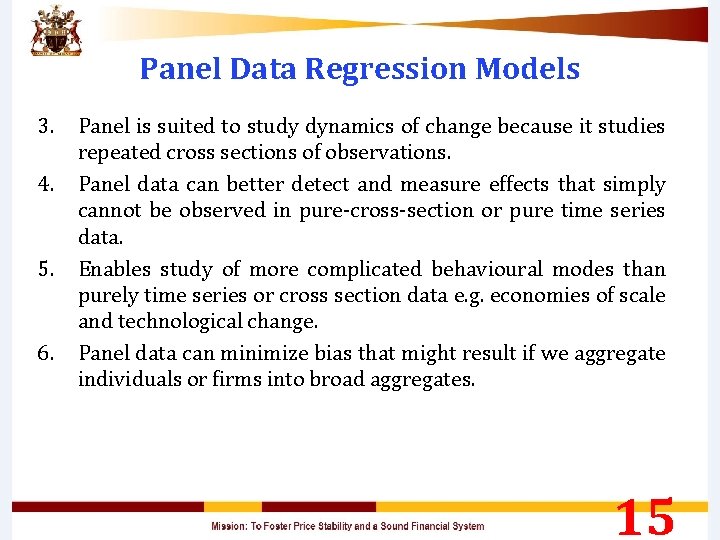
Panel Data Regression Models 3. 4. 5. 6. Panel is suited to study dynamics of change because it studies repeated cross sections of observations. Panel data can better detect and measure effects that simply cannot be observed in pure-cross-section or pure time series data. Enables study of more complicated behavioural modes than purely time series or cross section data e. g. economies of scale and technological change. Panel data can minimize bias that might result if we aggregate individuals or firms into broad aggregates. 15

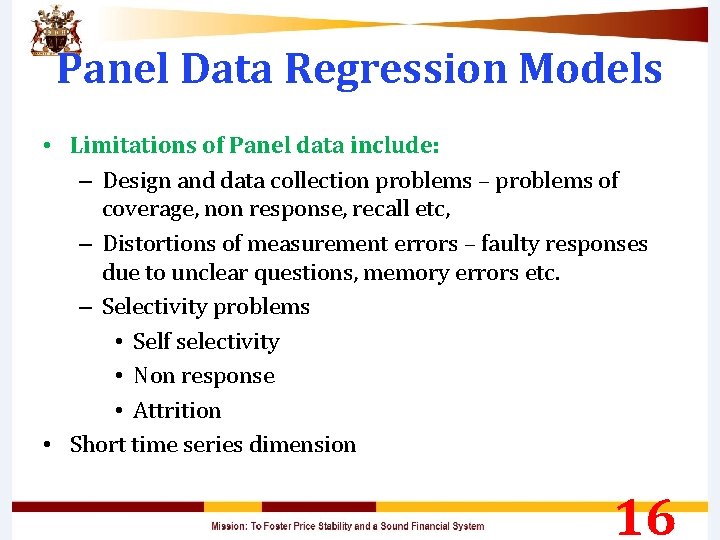
Panel Data Regression Models • Limitations of Panel data include: – Design and data collection problems – problems of coverage, non response, recall etc, – Distortions of measurement errors – faulty responses due to unclear questions, memory errors etc. – Selectivity problems • Self selectivity • Non response • Attrition • Short time series dimension 16

Panel Data Regression Models EXAMPLE • Non performing loans depend on loan to asset ratio and macroeconomic variables. For four banks BOB, BOA, CITI and DFCU. 1993 -2013. 17

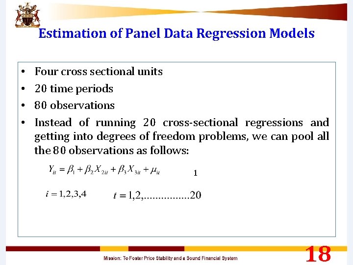
Estimation of Panel Data Regression Models • • Four cross sectional units 20 time periods 80 observations Instead of running 20 cross-sectional regressions and getting into degrees of freedom problems, we can pool all the 80 observations as follows: 1 18

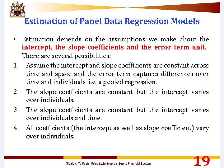
Estimation of Panel Data Regression Models • Estimation depends on the assumptions we make about the intercept, the slope coefficients and the error term unit. There are several possibilities: 1. Assume the intercept and slope coefficients are constant across time and space and the error term captures differences over time and individuals i. e. a pooled regression. 2. The slope coefficients are constant but the intercept varies over individuals. 3. The slope coefficients are constant but the intercept varies over individuals and time. 4. All coefficients (the intercept as well as slope coefficient) vary over individuals. 19

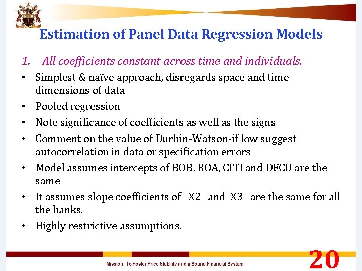
Estimation of Panel Data Regression Models 1. All coefficients constant across time and individuals. • Simplest & naïve approach, disregards space and time dimensions of data • Pooled regression • Note significance of coefficients as well as the signs • Comment on the value of Durbin-Watson-if low suggest autocorrelation in data or specification errors • Model assumes intercepts of BOB, BOA, CITI and DFCU are the same • It assumes slope coefficients of X 2 and X 3 are the same for all the banks. • Highly restrictive assumptions. 20

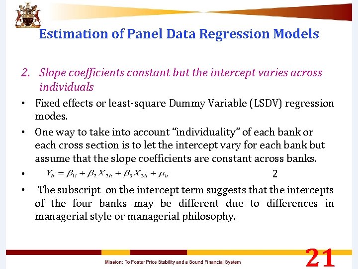
Estimation of Panel Data Regression Models 2. Slope coefficients constant but the intercept varies across individuals • Fixed effects or least-square Dummy Variable (LSDV) regression modes. • One way to take into account “individuality” of each bank or each cross section is to let the intercept vary for each bank but assume that the slope coefficients are constant across banks. • 2 • The subscript on the intercept term suggests that the intercepts of the four banks may be different due to differences in managerial style or managerial philosophy. 21

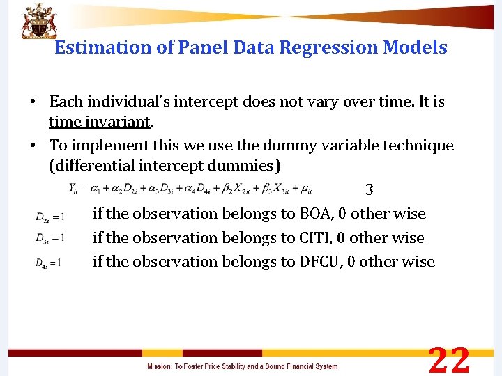
Estimation of Panel Data Regression Models • Each individual’s intercept does not vary over time. It is time invariant. • To implement this we use the dummy variable technique (differential intercept dummies) 3 if the observation belongs to BOA, 0 other wise if the observation belongs to CITI, 0 other wise if the observation belongs to DFCU, 0 other wise 22

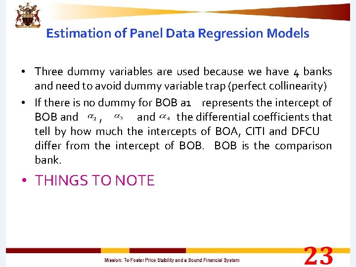
Estimation of Panel Data Regression Models • Three dummy variables are used because we have 4 banks and need to avoid dummy variable trap (perfect collinearity) • If there is no dummy for BOB a 1 represents the intercept of BOB and , and the differential coefficients that tell by how much the intercepts of BOA, CITI and DFCU differ from the intercept of BOB is the comparison bank. • THINGS TO NOTE 23

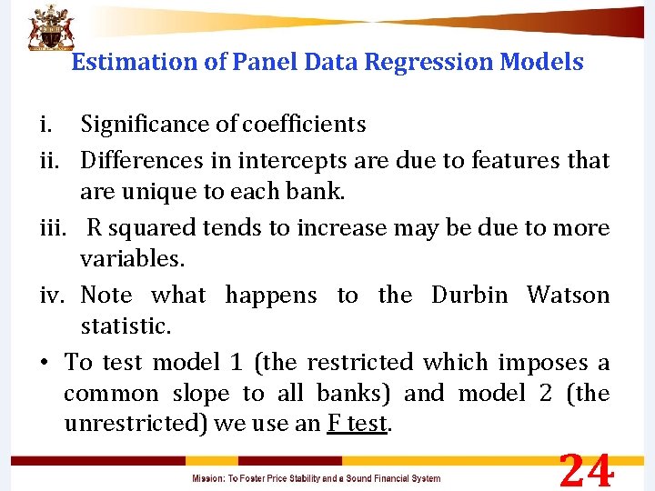
Estimation of Panel Data Regression Models i. Significance of coefficients ii. Differences in intercepts are due to features that are unique to each bank. iii. R squared tends to increase may be due to more variables. iv. Note what happens to the Durbin Watson statistic. • To test model 1 (the restricted which imposes a common slope to all banks) and model 2 (the unrestricted) we use an F test. 24

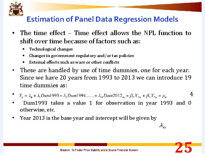
Estimation of Panel Data Regression Models • The time effect – Time effect allows the NPL function to shift over time because of factors such as: § Technological changes § Changes in government regulatory and/or tax policies § External effects such as wars or other conflicts • These are handled by use of time dummies, one for each year. Since we have 20 years from 1993 to 2013 we can introduce 19 time dummies as: • 4 • Dum 1993 takes a value 1 for observation in year 1993 and 0 otherwise, etc. • Year 2013 is the base year and intercept will be given by 25

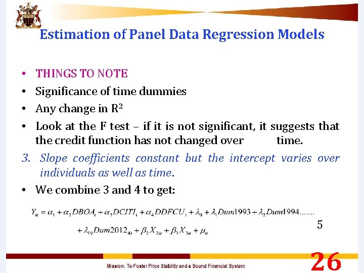
Estimation of Panel Data Regression Models THINGS TO NOTE Significance of time dummies Any change in R 2 Look at the F test – if it is not significant, it suggests that the credit function has not changed over time. 3. Slope coefficients constant but the intercept varies over individuals as well as time. • We combine 3 and 4 to get: • • 5 26

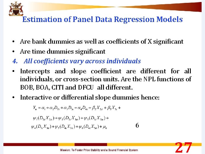
Estimation of Panel Data Regression Models Are bank dummies as well as coefficients of X significant Are time dummies significant All coefficients vary across individuals Intercepts and slope coefficient are different for all individuals, or cross-section units. Are the NPL functions of BOB, BOA, CITI and DFCU all different. • Interactive or differential slope dummies hence: • • 4. • 6 27

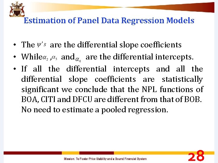
Estimation of Panel Data Regression Models • The are the differential slope coefficients • While , and are the differential intercepts. • If all the differential intercepts and all the differential slope coefficients are statistically significant we conclude that the NPL functions of BOA, CITI and DFCU are different from that of BOB. No need to estimate a pooled regression. 28

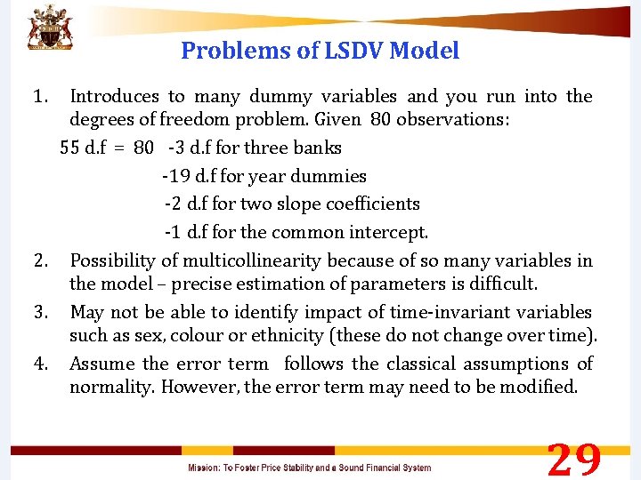
Problems of LSDV Model 1. Introduces to many dummy variables and you run into the degrees of freedom problem. Given 80 observations: 55 d. f = 80 -3 d. f for three banks -19 d. f for year dummies -2 d. f for two slope coefficients -1 d. f for the common intercept. 2. Possibility of multicollinearity because of so many variables in the model – precise estimation of parameters is difficult. 3. May not be able to identify impact of time-invariant variables such as sex, colour or ethnicity (these do not change over time). 4. Assume the error term follows the classical assumptions of normality. However, the error term may need to be modified. 29

Estimation of Panel Data Regression Models • The One way error component model – The Fixed Effects Model – The Random Effects Model • The two way Error Component Model – The Fixed Effects Model – The Random Effects Model 30

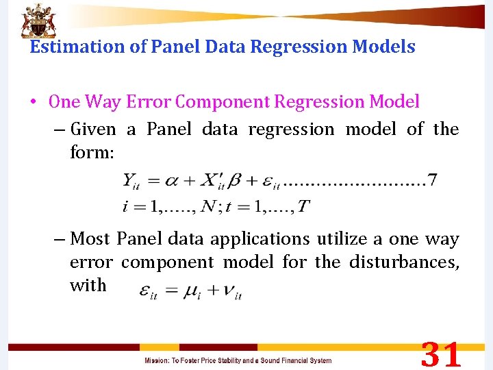
Estimation of Panel Data Regression Models • One Way Error Component Regression Model – Given a Panel data regression model of the form: – Most Panel data applications utilize a one way error component model for the disturbances, with 31

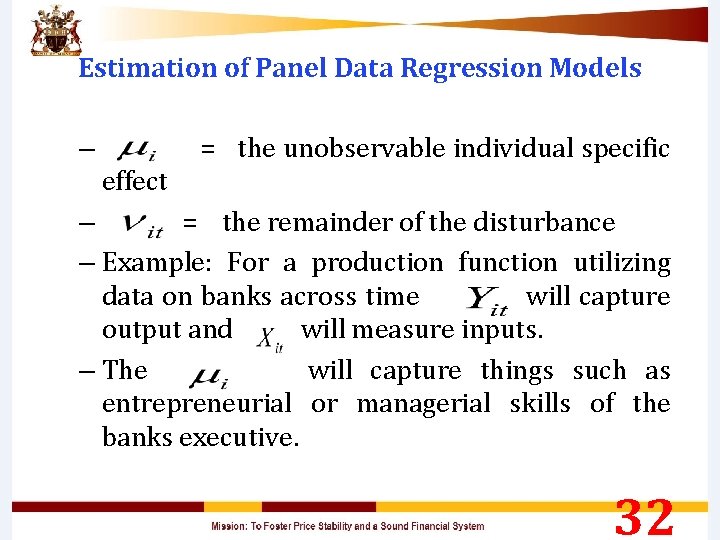
Estimation of Panel Data Regression Models – = the unobservable individual specific effect – = the remainder of the disturbance – Example: For a production function utilizing data on banks across time will capture output and will measure inputs. – The will capture things such as entrepreneurial or managerial skills of the banks executive. 32

Estimation of Panel Data Regression Models • The Fixed Effects Model – In this model the are assumed to be fixed effects to be estimated and the remainder disturbances are stochastic with independent and identically distributed – for all and . 33

Estimation of Panel Data Regression Models • This model is appropriate when inference is restricted to a specific set of Known firms whose behavior we are interested in. • The Fixed Effects (FE) Least Squares is also known as the Least Squares Dummy Variables (LSDV). 34

Estimation of Panel Data Regression Models • The Random Effects Model – There too many parameters in the fixed effects model and the loss of degrees of freedom can be avoided if is assumed to be random. In this case: – and are independent of . 35

Estimation of Panel Data Regression Models – In addition, the are independent of the and for all and . – The random effects model is an appropriate specification if we are drawing individuals randomly from a large population. – The individual effect is characterized as random and inference pertains to the population that the sample was randomly drawn. 36

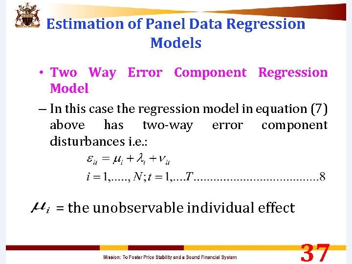
Estimation of Panel Data Regression Models • Two Way Error Component Regression Model – In this case the regression model in equation (7) above has two-way error component disturbances i. e. : = the unobservable individual effect 37

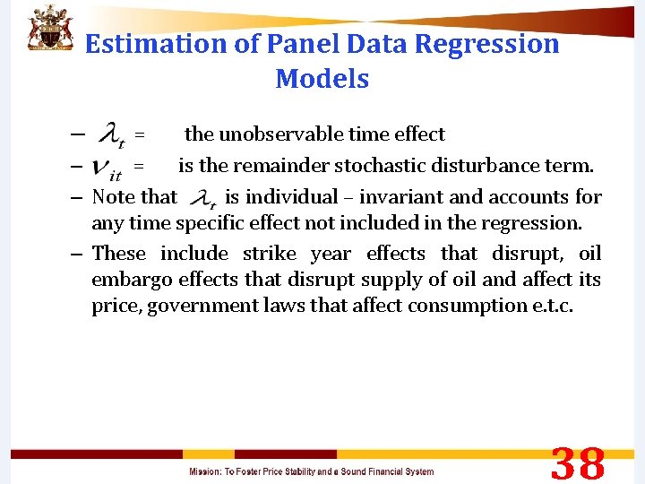
Estimation of Panel Data Regression Models – = the unobservable time effect – = is the remainder stochastic disturbance term. – Note that is individual – invariant and accounts for any time specific effect not included in the regression. – These include strike year effects that disrupt, oil embargo effects that disrupt supply of oil and affect its price, government laws that affect consumption e. t. c. 38

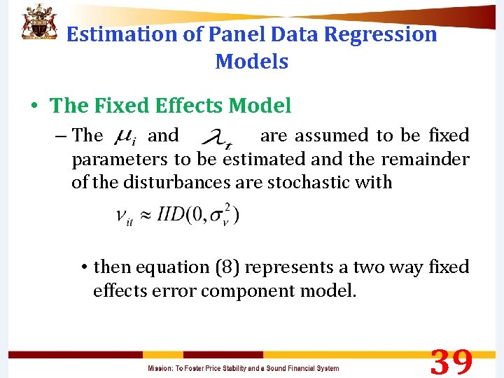
Estimation of Panel Data Regression Models • The Fixed Effects Model – The and are assumed to be fixed parameters to be estimated and the remainder of the disturbances are stochastic with • then equation (8) represents a two way fixed effects error component model. 39

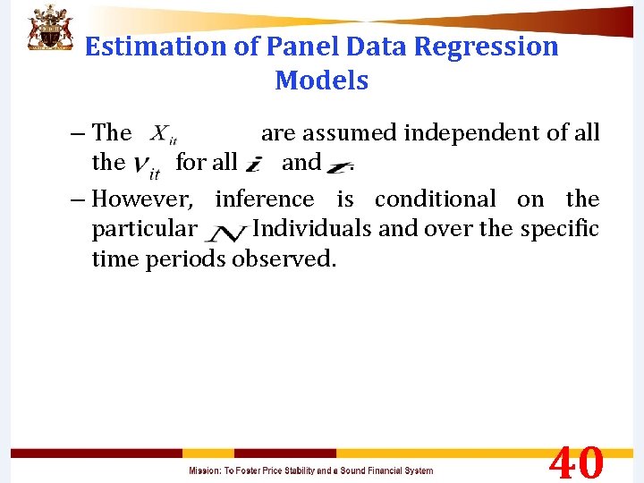
Estimation of Panel Data Regression Models – The are assumed independent of all the for all and . – However, inference is conditional on the particular Individuals and over the specific time periods observed. 40

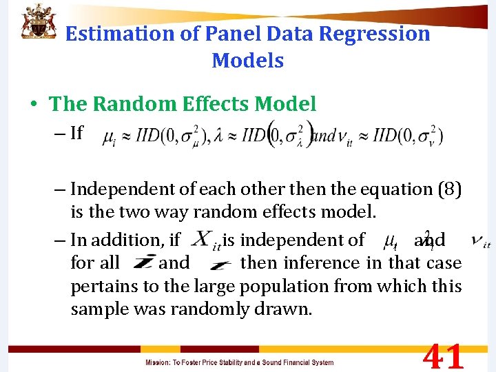
Estimation of Panel Data Regression Models • The Random Effects Model – If – Independent of each other then the equation (8) is the two way random effects model. – In addition, if is independent of , and for all and then inference in that case pertains to the large population from which this sample was randomly drawn. 41

SOME PRACTICAL APPLICATIONS WITH UGANDAN DATA 42

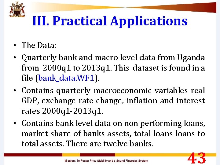
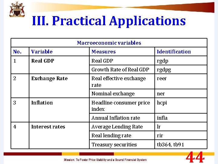
III. Practical Applications • The Data: • Quarterly bank and macro level data from Uganda from 2000 q 1 to 2013 q 1. This dataset is found in a file (bank_data. WF 1). • Contains quarterly macroeconomic variables real GDP, exchange rate change, inflation and interest rates 2000 q 1 -2013 q 1. • Contains bank level data on non performing loans, market share of banks assets, total loans to total assets. There are twelve banks. 43

III. Practical Applications Macroeconomic variables No. Variable Measures Identification 1 Real GDP rgdp Growth Rate of Real GDP rgdpg Real effective exchange rate reer Nominal exchange ner Headline consumer price index hcpi Annual Inflation rate infla Average Lending Rate lr Real lending rate rir Treasury securities tb 364, tb 91 2 3 4 Exchange Rate Inflation Interest rates 44

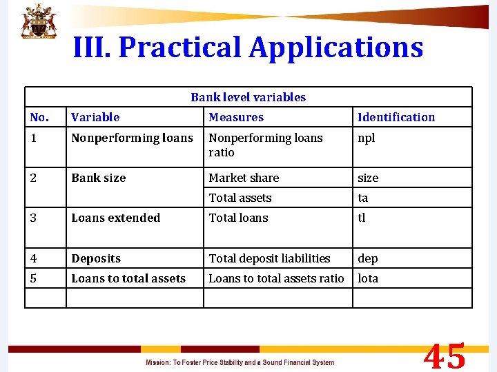
III. Practical Applications Bank level variables No. Variable Measures Identification 1 Nonperforming loans ratio npl 2 Bank size Market share size Total assets ta 3 Loans extended Total loans tl 4 Deposits Total deposit liabilities dep 5 Loans to total assets ratio lota 45

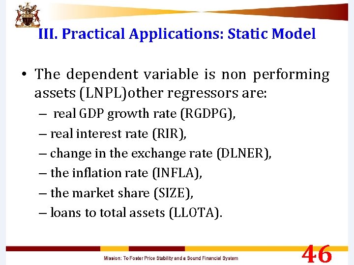
III. Practical Applications: Static Model • The dependent variable is non performing assets (LNPL)other regressors are: – real GDP growth rate (RGDPG), – real interest rate (RIR), – change in the exchange rate (DLNER), – the inflation rate (INFLA), – the market share (SIZE), – loans to total assets (LLOTA). 46

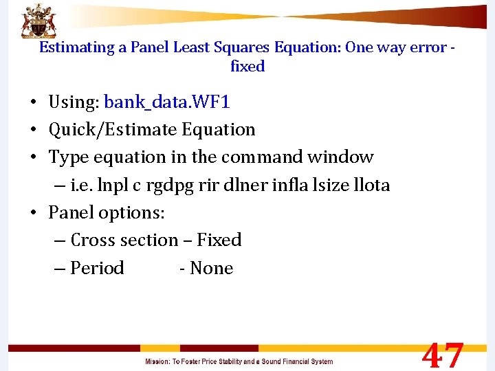
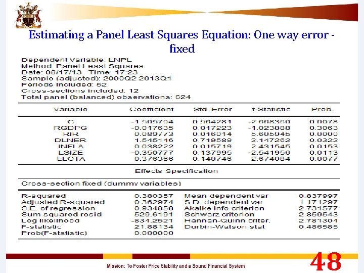
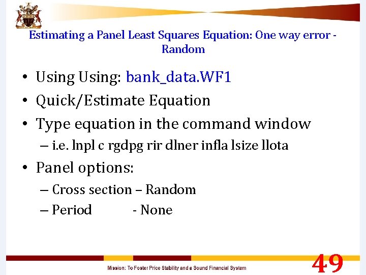
Estimating a Panel Least Squares Equation: One way error - fixed • Using: bank_data. WF 1 • Quick/Estimate Equation • Type equation in the command window – i. e. lnpl c rgdpg rir dlner infla lsize llota • Panel options: – Cross section – Fixed – Period - None 47

Estimating a Panel Least Squares Equation: One way error - fixed 48

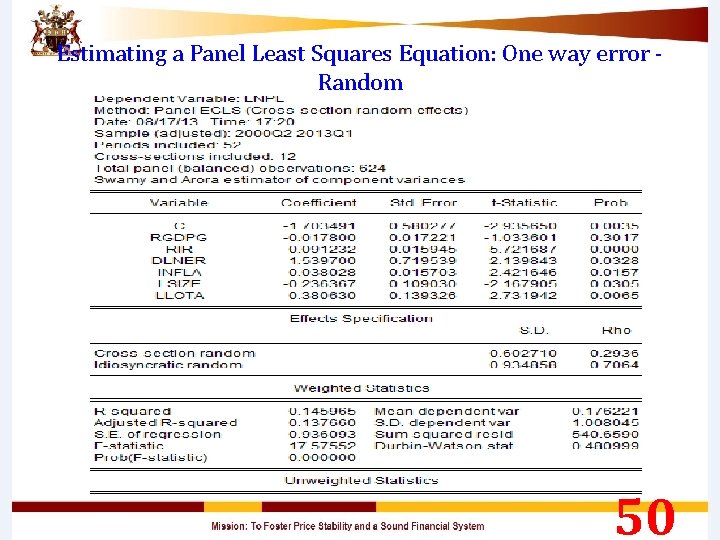
Estimating a Panel Least Squares Equation: One way error - Random • Using: bank_data. WF 1 • Quick/Estimate Equation • Type equation in the command window – i. e. lnpl c rgdpg rir dlner infla lsize llota • Panel options: – Cross section – Random – Period - None 49

Estimating a Panel Least Squares Equation: One way error - Random 50

Estimating a Panel Least Squares Equation: Two way error - Fixed • Will not be estimated, nature of the data set. 51

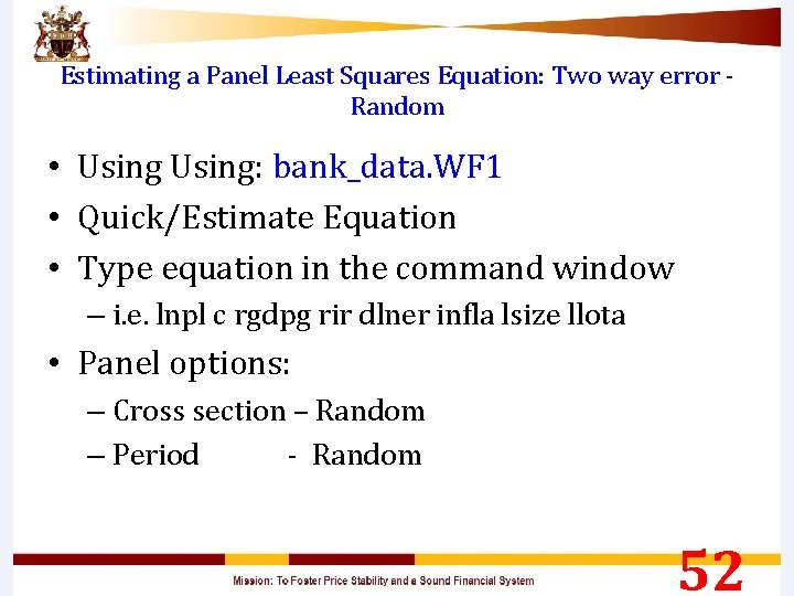
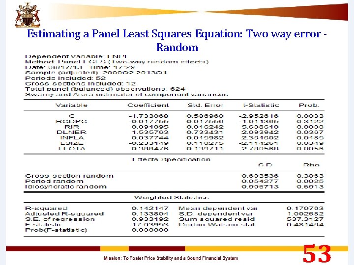
Estimating a Panel Least Squares Equation: Two way error - Random • Using: bank_data. WF 1 • Quick/Estimate Equation • Type equation in the command window – i. e. lnpl c rgdpg rir dlner infla lsize llota • Panel options: – Cross section – Random – Period - Random 52

Estimating a Panel Least Squares Equation: Two way error - Random 53

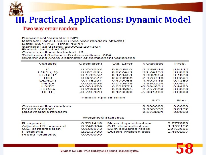
III. Practical Applications: Dynamic Model • Estimate a dynamic panel least equations using: – The nonperforming assets ratio (LNPL) and other regressors such namely regressors are • • lagged NPL ratio (LNPL(-1), real GDP rate (LRGDP), RGDPG real interest rate (RIR), LTB 364, LTB 91, LR change in the exchange rate (DLNER), LREER the inflation rate (INFLA), LHCPL, DLHCPI the market share (SIZE), loans to total assets (LLOTA), LTA growth in total loans (DLTL). LTL 54

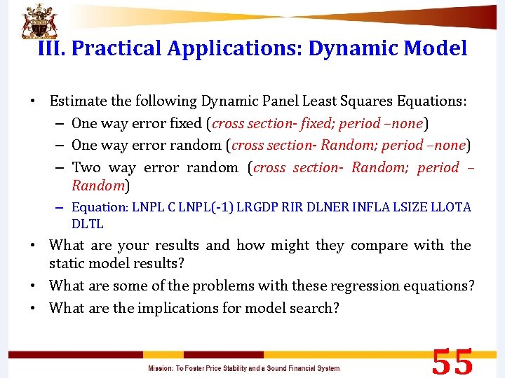
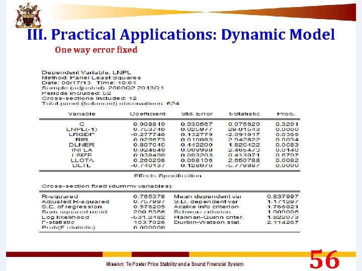
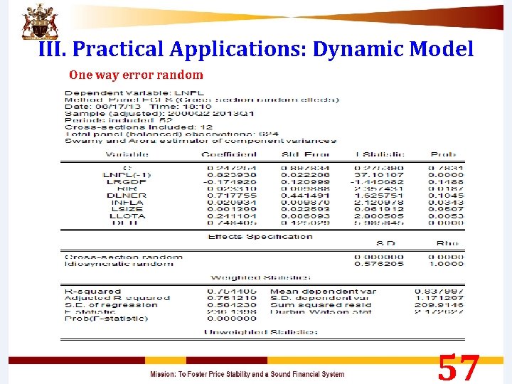
III. Practical Applications: Dynamic Model • Estimate the following Dynamic Panel Least Squares Equations: – One way error fixed (cross section- fixed; period –none) – One way error random (cross section- Random; period –none) – Two way error random (cross section- Random; period – Random) – Equation: LNPL C LNPL(-1) LRGDP RIR DLNER INFLA LSIZE LLOTA DLTL • What are your results and how might they compare with the static model results? • What are some of the problems with these regression equations? • What are the implications for model search? 55

III. Practical Applications: Dynamic Model One way error fixed 56

III. Practical Applications: Dynamic Model One way error random 57

III. Practical Applications: Dynamic Model Two way error random 58

FURTHER TOPICS 59

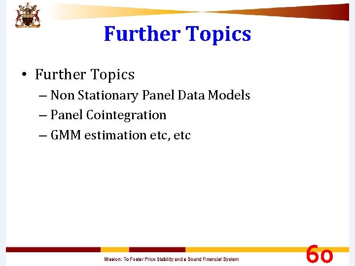
Further Topics • Further Topics – Non Stationary Panel Data Models – Panel Cointegration – GMM estimation etc, etc 60

REFERENCES 61

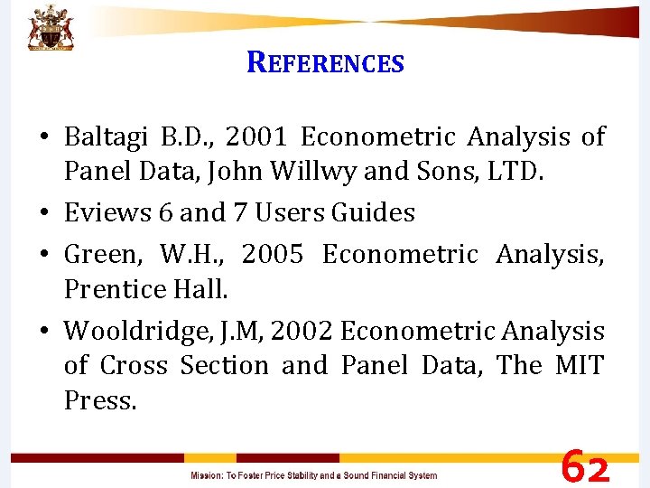
REFERENCES • Baltagi B. D. , 2001 Econometric Analysis of Panel Data, John Willwy and Sons, LTD. • Eviews 6 and 7 Users Guides • Green, W. H. , 2005 Econometric Analysis, Prentice Hall. • Wooldridge, J. M, 2002 Econometric Analysis of Cross Section and Panel Data, The MIT Press. 62