load fisheriris x meas 3 4 gscatterx 1

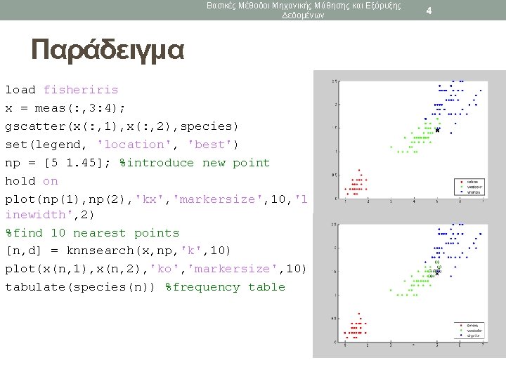
Βασικές Μέθοδοι Μηχανικής Μάθησης και Εξόρυξης Δεδομένων Παράδειγμα load fisheriris x = meas(: , 3: 4); gscatter(x(: , 1), x(: , 2), species) set(legend, 'location', 'best') np = [5 1. 45]; %introduce new point hold on plot(np(1), np(2), 'kx', 'markersize', 10, 'l inewidth', 2) %find 10 nearest points [n, d] = knnsearch(x, np, 'k', 10) plot(x(n, 1), x(n, 2), 'ko', 'markersize', 10) tabulate(species(n)) %frequency table 4

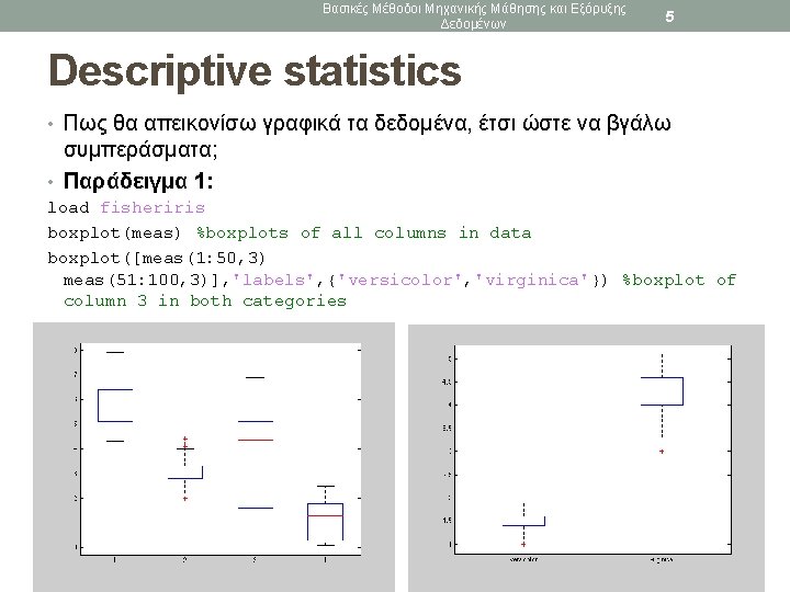
Βασικές Μέθοδοι Μηχανικής Μάθησης και Εξόρυξης Δεδομένων 5 Descriptive statistics • Πως θα απεικονίσω γραφικά τα δεδομένα, έτσι ώστε να βγάλω συμπεράσματα; • Παράδειγμα 1: load fisheriris boxplot(meas) %boxplots of all columns in data boxplot([meas(1: 50, 3) meas(51: 100, 3)], 'labels', {'versicolor', 'virginica'}) %boxplot of column 3 in both categories

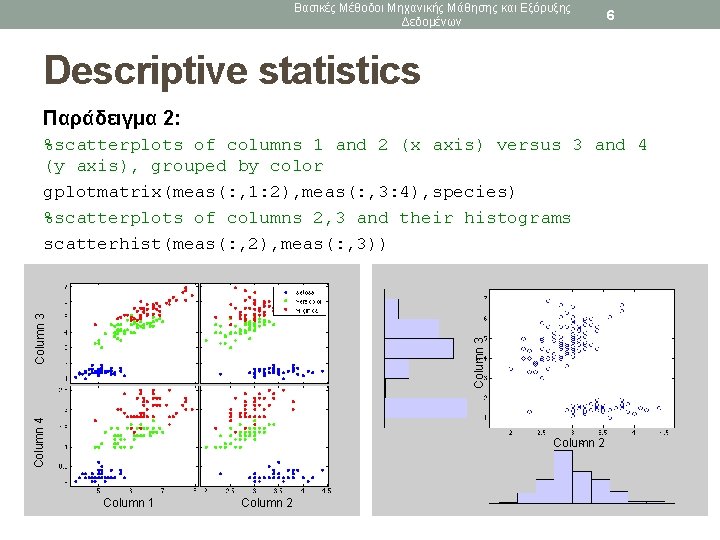
Βασικές Μέθοδοι Μηχανικής Μάθησης και Εξόρυξης Δεδομένων 6 Descriptive statistics Παράδειγμα 2: Column 4 Column 3 %scatterplots of columns 1 and 2 (x axis) versus 3 and 4 (y axis), grouped by color gplotmatrix(meas(: , 1: 2), meas(: , 3: 4), species) %scatterplots of columns 2, 3 and their histograms scatterhist(meas(: , 2), meas(: , 3)) Column 2 Column 1 Column 2

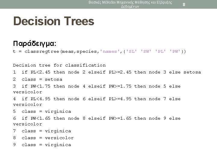
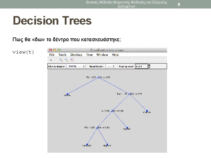
Βασικές Μέθοδοι Μηχανικής Μάθησης και Εξόρυξης Δεδομένων 8 Decision Trees Παράδειγμα: t = classregtree(meas, species, 'names', {'SL' 'SW' 'PL' 'PW'}) Decision tree for classification 1 if PL<2. 45 then node 2 elseif 2 class = setosa 3 if PW<1. 75 then node 4 elseif versicolor 4 if PL<4. 95 then node 6 elseif versicolor 5 class = virginica 6 if PW<1. 65 then node 8 elseif versicolor 7 class = virginica 8 class = versicolor 9 class = virginica PL>=2. 45 then node 3 else setosa PW>=1. 75 then node 5 else PL>=4. 95 then node 7 else PW>=1. 65 then node 9 else

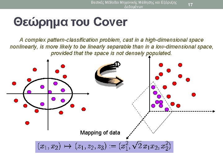
Βασικές Μέθοδοι Μηχανικής Μάθησης και Εξόρυξης Δεδομένων 17 Θεώρημα του Cover A complex pattern-classification problem, cast in a high-dimensional space nonlinearly, is more likely to be linearly separable than in a low-dimensional space, provided that the space is not densely populated. Mapping of data

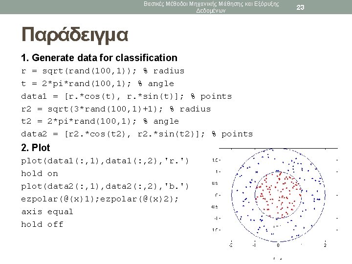
Βασικές Μέθοδοι Μηχανικής Μάθησης και Εξόρυξης Δεδομένων Παράδειγμα 1. Generate data for classification r = sqrt(rand(100, 1)); % radius t = 2*pi*rand(100, 1); % angle data 1 = [r. *cos(t), r. *sin(t)]; % points r 2 = sqrt(3*rand(100, 1)+1); % radius t 2 = 2*pi*rand(100, 1); % angle data 2 = [r 2. *cos(t 2), r 2. *sin(t 2)]; % points 2. Plot plot(data 1(: , 1), data 1(: , 2), 'r. ') hold on plot(data 2(: , 1), data 2(: , 2), 'b. ') ezpolar(@(x)1); ezpolar(@(x)2); axis equal hold off 23

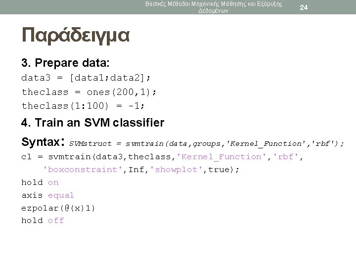
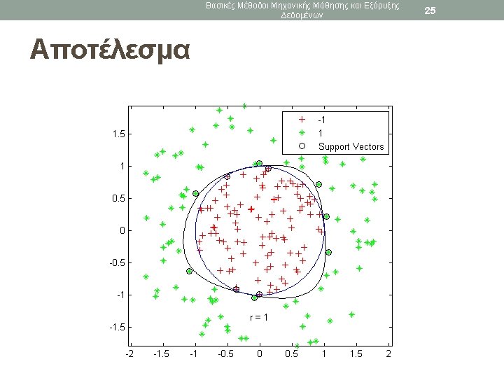
Βασικές Μέθοδοι Μηχανικής Μάθησης και Εξόρυξης Δεδομένων 24 Παράδειγμα 3. Prepare data: data 3 = [data 1; data 2]; theclass = ones(200, 1); theclass(1: 100) = -1; 4. Train an SVM classifier Syntax: SVMstruct = svmtrain(data, groups, 'Kernel_Function', 'rbf'); cl = svmtrain(data 3, theclass, 'Kernel_Function', 'rbf', 'boxconstraint', Inf, 'showplot', true); hold on axis equal ezpolar(@(x)1) hold off

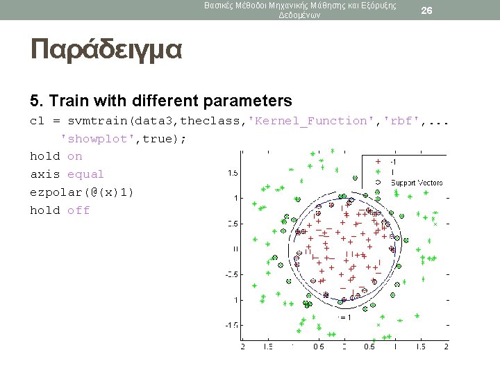
Βασικές Μέθοδοι Μηχανικής Μάθησης και Εξόρυξης Δεδομένων 26 Παράδειγμα 5. Train with different parameters cl = svmtrain(data 3, theclass, 'Kernel_Function', 'rbf', . . . 'showplot', true); hold on axis equal ezpolar(@(x)1) hold off