Lecture 7 Liquidity Liquidity Concepts Liquidity is like

Lecture 7 Liquidity

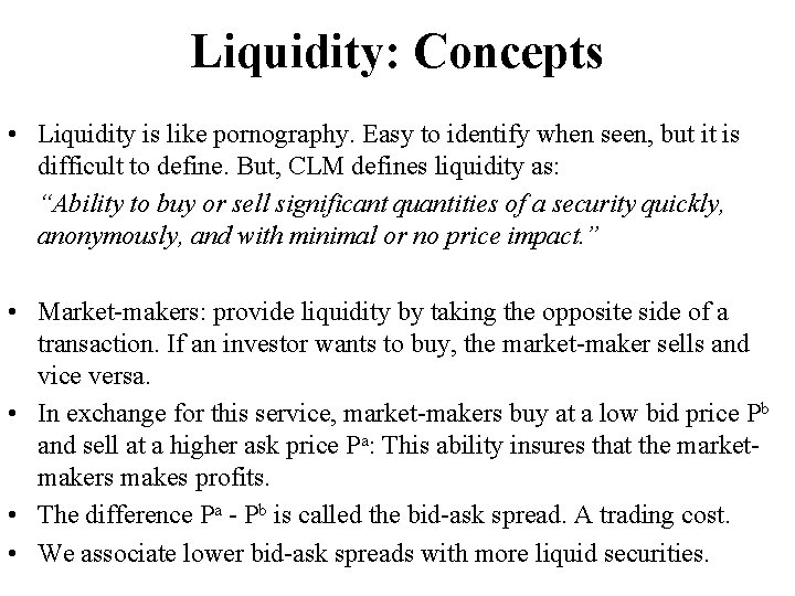
Liquidity: Concepts • Liquidity is like pornography. Easy to identify when seen, but it is difficult to define. But, CLM defines liquidity as: “Ability to buy or sell significant quantities of a security quickly, anonymously, and with minimal or no price impact. ” • Market-makers: provide liquidity by taking the opposite side of a transaction. If an investor wants to buy, the market-maker sells and vice versa. • In exchange for this service, market-makers buy at a low bid price Pb and sell at a higher ask price Pa: This ability insures that the marketmakers makes profits. • The difference Pa - Pb is called the bid-ask spread. A trading cost. • We associate lower bid-ask spreads with more liquid securities.

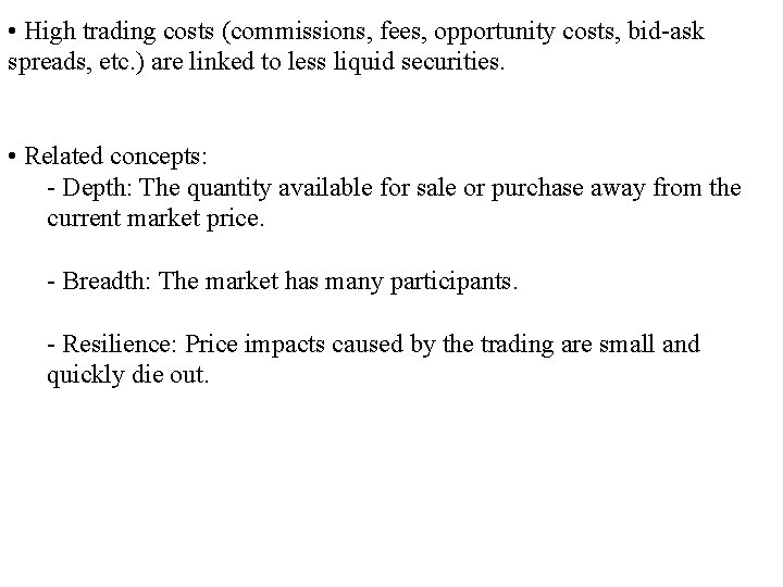
• High trading costs (commissions, fees, opportunity costs, bid-ask spreads, etc. ) are linked to less liquid securities. • Related concepts: - Depth: The quantity available for sale or purchase away from the current market price. - Breadth: The market has many participants. - Resilience: Price impacts caused by the trading are small and quickly die out.

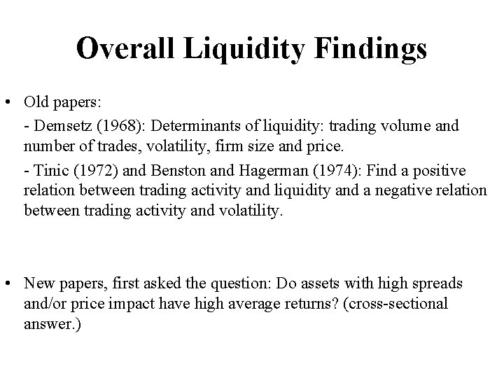
Overall Liquidity Findings • Old papers: - Demsetz (1968): Determinants of liquidity: trading volume and number of trades, volatility, firm size and price. - Tinic (1972) and Benston and Hagerman (1974): Find a positive relation between trading activity and liquidity and a negative relation between trading activity and volatility. • New papers, first asked the question: Do assets with high spreads and/or price impact have high average returns? (cross-sectional answer. )

Findings: Positive relationship between expected stock returns and alternative proxies for individual illiquidity levels - Amihud and Mendelson (1986) –bid-ask spreads-, Brennan and Subrahmanyan (1996) –price impacts- Datar et al. (1998) –bid-asks spreads-, Easley et al. (EHO) (2002) - PINs. • Second, papers study the time series properties of aggregate liquidity measures. Findings: Existence of predictability and commonality in liquidity Chordia, Roll and Subrahmanyam (2001), Hasbrouck and Seppi (2001), Amihud (2002), Jones (2002), Huberman and Halka (2001).

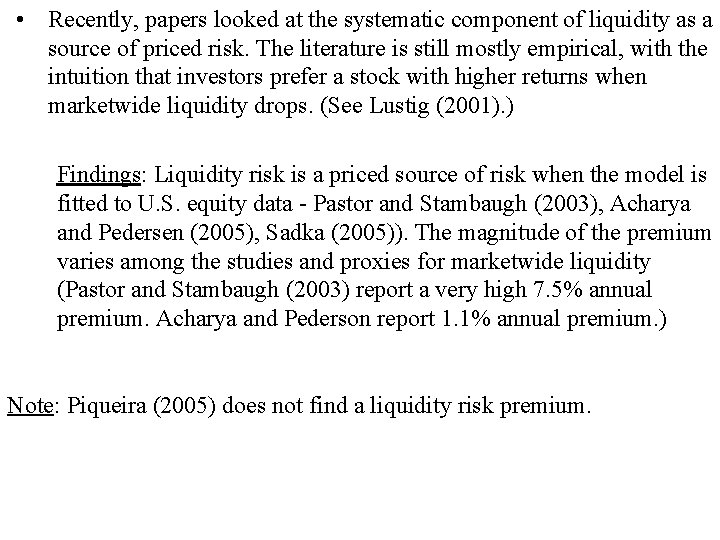
• Recently, papers looked at the systematic component of liquidity as a source of priced risk. The literature is still mostly empirical, with the intuition that investors prefer a stock with higher returns when marketwide liquidity drops. (See Lustig (2001). ) Findings: Liquidity risk is a priced source of risk when the model is fitted to U. S. equity data - Pastor and Stambaugh (2003), Acharya and Pedersen (2005), Sadka (2005)). The magnitude of the premium varies among the studies and proxies for marketwide liquidity (Pastor and Stambaugh (2003) report a very high 7. 5% annual premium. Acharya and Pederson report 1. 1% annual premium. ) Note: Piqueira (2005) does not find a liquidity risk premium.

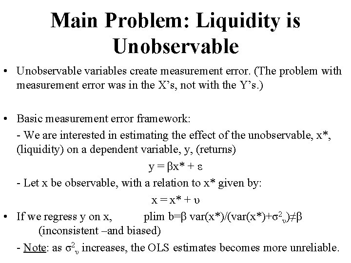
Main Problem: Liquidity is Unobservable • Unobservable variables create measurement error. (The problem with measurement error was in the X’s, not with the Y’s. ) • Basic measurement error framework: - We are interested in estimating the effect of the unobservable, x*, (liquidity) on a dependent variable, y, (returns) y = βx* + ε - Let x be observable, with a relation to x* given by: x = x* + υ • If we regress y on x, plim b=β var(x*)/(var(x*)+σ2υ)≠β (inconsistent –and biased) - Note: as σ2υ increases, the OLS estimates becomes more unreliable.

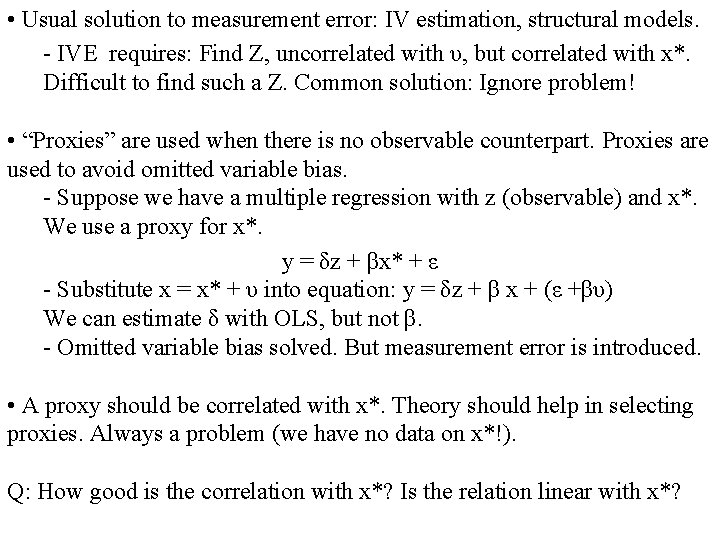
• Usual solution to measurement error: IV estimation, structural models. - IVE requires: Find Z, uncorrelated with υ, but correlated with x*. Difficult to find such a Z. Common solution: Ignore problem! • “Proxies” are used when there is no observable counterpart. Proxies are used to avoid omitted variable bias. - Suppose we have a multiple regression with z (observable) and x*. We use a proxy for x*. y = δz + βx* + ε - Substitute x = x* + υ into equation: y = δz + β x + (ε +βυ) We can estimate δ with OLS, but not β. - Omitted variable bias solved. But measurement error is introduced. • A proxy should be correlated with x*. Theory should help in selecting proxies. Always a problem (we have no data on x*!). Q: How good is the correlation with x*? Is the relation linear with x*?

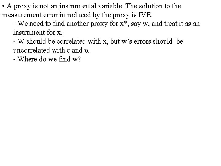
• A proxy is not an instrumental variable. The solution to the measurement error introduced by the proxy is IVE. - We need to find another proxy for x*, say w, and treat it as an instrument for x. - W should be correlated with x, but w’s errors should be uncorrelated with ε and υ. - Where do we find w?

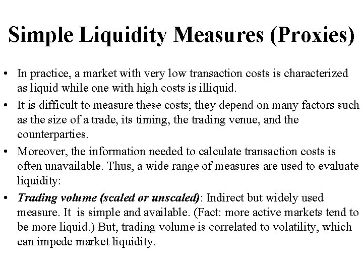
Simple Liquidity Measures (Proxies) • In practice, a market with very low transaction costs is characterized as liquid while one with high costs is illiquid. • It is difficult to measure these costs; they depend on many factors such as the size of a trade, its timing, the trading venue, and the counterparties. • Moreover, the information needed to calculate transaction costs is often unavailable. Thus, a wide range of measures are used to evaluate liquidity: • Trading volume (scaled or unscaled): Indirect but widely used measure. It is simple and available. (Fact: more active markets tend to be more liquid. ) But, trading volume is correlated to volatility, which can impede market liquidity.

• Trading frequency: Number of trades executed within a specified interval, without regard to trade size. High trading frequency may also indicate a more liquid market, but it too can be associated with volatility and hence lower liquidity. • The bid-ask spread (Level or %): It measures the cost of executing a small trade. Usually calculated as the difference between the bid or offer price and the bid-ask midpoint. It can be calculated quickly, with data widely available in real time. But, bid and offer quotes are good only for limited quantities and time periods; the spread just measures the cost of executing a single trade of a certain size. • Quote size: Quantity of securities tradable at the bid and offer prices. It accounts for market depth and complements the bid-ask spread. Market makers often do not reveal the full quantities they will transact at a given price, so the measured depth underestimates the true depth.

• Trade size: Quantity of securities traded at the bid and offer prices, reflecting any negotiation over quantity. Alternative depth measure. Trade size also underestimates market depth, because the quantity traded is often less than the quantity that could have been traded at a given price. • Price impact coefficient (Temporary or Permanent): It considers the rise (fall) in price that typically occurs with a buyer-initiated (sellerinitiated) trade. Useful for large trades or a series of trades. Together with the bid-ask spread and depth measures provides a good picture of liquidity. A drawback is the difficulty of obtaining the data required for estimation, particularly on a real-time basis.

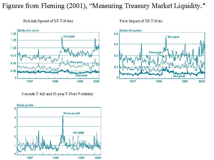
Figures from Fleming (2001), “Measuring Treasury Market Liquidity. ” Bid-Ask Spread of US T-Notes 3 -month T-bill and 10 -year T-Note Volatility Price Impact of US T-Nots

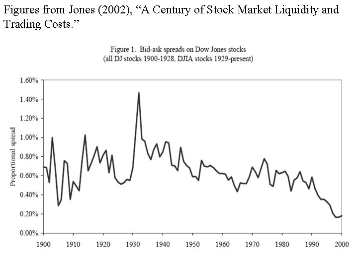
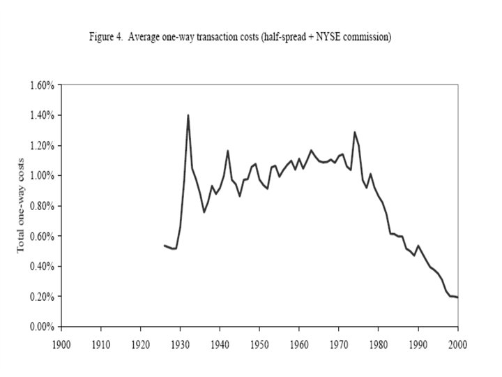
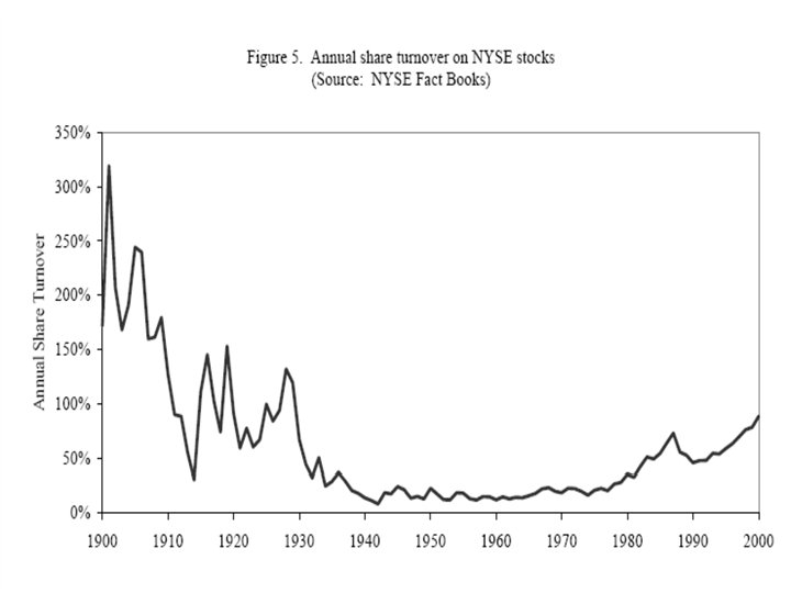
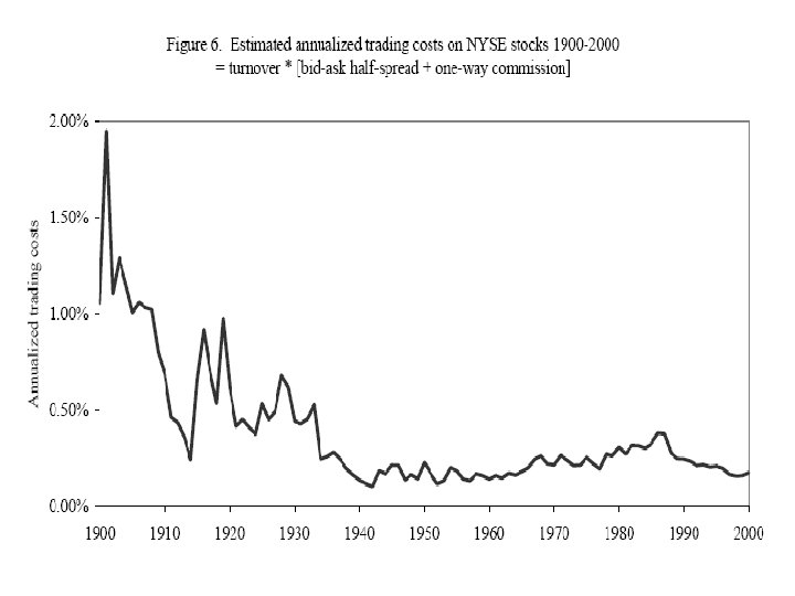
Figures from Jones (2002), “A Century of Stock Market Liquidity and Trading Costs. ”

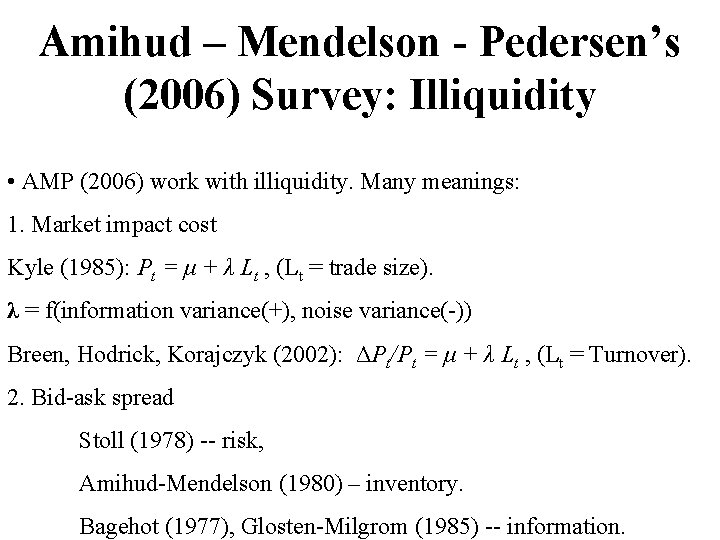
Amihud – Mendelson - Pedersen’s (2006) Survey: Illiquidity • AMP (2006) work with illiquidity. Many meanings: 1. Market impact cost Kyle (1985): Pt = μ + λ Lt , (Lt = trade size). λ = f(information variance(+), noise variance(-)) Breen, Hodrick, Korajczyk (2002): ΔPt/Pt = μ + λ Lt , (Lt = Turnover). 2. Bid-ask spread Stoll (1978) -- risk, Amihud-Mendelson (1980) – inventory. Bagehot (1977), Glosten-Milgrom (1985) -- information.

3. Search and delay costs, price and execution risk. 4. Commissions, fees, cost of time, etc.

Liquidity Levels Premium (crosssection) • Amihud and Mendelson (1986): Microstructure Equilibrium Model. Negative relation between transaction costs (S, %) and stock prices. • In equilibrium: 1. Investors choose assets depending on the (Sj). If an investor is willing to hold stocks for a long period, the investor is willing to buy high Sj stocks. (Liquidity clientele. ) 2. Model links: (i) Expected return and spread (ii) Expected return and turnover (reflecting holding period differences. ) Findings: using 49 stock portfolios, sorted by β and S, updating the grouping every year and looking at returns one year ahead. Example: Ri = 0. 0065 + 0. 01⋅βi + 0. 0021⋅log(Si)

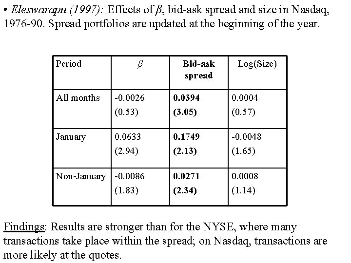
• Eleswarapu (1997): Effects of β, bid-ask spread and size in Nasdaq, 1976 -90. Spread portfolios are updated at the beginning of the year. Period β Bid-ask spread Log(Size) All months -0. 0026 (0. 53) 0. 0394 (3. 05) 0. 0004 (0. 57) January 0. 0633 (2. 94) 0. 1749 (2. 13) -0. 0048 (1. 65) 0. 0271 (2. 34) 0. 0008 (1. 14) Non-January -0. 0086 (1. 83) Findings: Results are stronger than for the NYSE, where many transactions take place within the spread; on Nasdaq, transactions are more likely at the quotes.

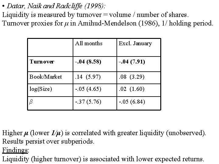
• Datar, Naik and Radcliffe (1998): Liquidity is measured by turnover = volume / number of shares. Turnover proxies for μ in Amihud-Mendelson (1986), 1/ holding period. All months Excl. January Turnover -. 04 (8. 58) -. 04 (7. 91) Book/Market . 14 (5. 97) . 08 (3. 29) log(Size) -. 05 (4. 65) . 02 (1. 60) β -. 37 (5. 76) -. 05 (6. 84) Higher μ (lower 1/μ) is correlated with greater liquidity (unobserved). Results persist over subperiods. Findings: Liquidity (higher turnover) is associated with lower expected returns.

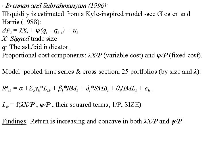
• Brennan and Subrahmanyam (1996): Illiquidity is estimated from a Kyle-inspired model -see Glosten and Harris (1988): ΔPt = λXt + ψ(qt – qt-1) + ut. X: Signed trade size q: The ask/bid indicator. Proportional cost components: λX/P (variable cost) and ψ/P (fixed cost). Model: pooled time series & cross section, 25 portfolios (by size and λ): Reit = α +Σkγk*Lik + βi*RMt + δi*SMBt + θi. HMLt + eit. Lik = f(λX/P , ψ/P , their squared terms, 1/P, SIZE). Findings: Return is increasing and concave in both λX/P and ψ/P.

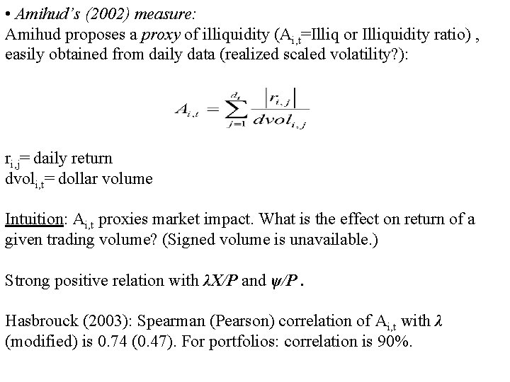
• Amihud’s (2002) measure: Amihud proposes a proxy of illiquidity (Ai, t=Illiq or Illiquidity ratio) , easily obtained from daily data (realized scaled volatility? ): ri, j= daily return dvoli, t= dollar volume Intuition: Ai, t proxies market impact. What is the effect on return of a given trading volume? (Signed volume is unavailable. ) Strong positive relation with λX/P and ψ/P. Hasbrouck (2003): Spearman (Pearson) correlation of Ai, t with λ (modified) is 0. 74 (0. 47). For portfolios: correlation is 90%.

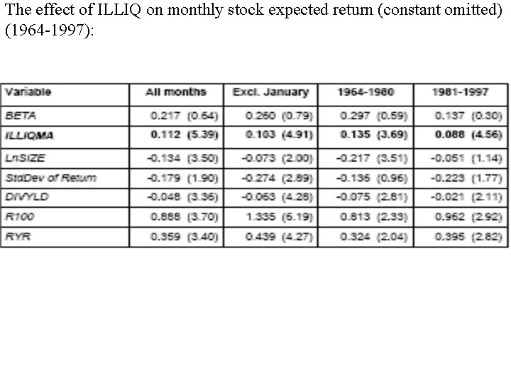
The effect of ILLIQ on monthly stock expected return (constant omitted) (1964 -1997):

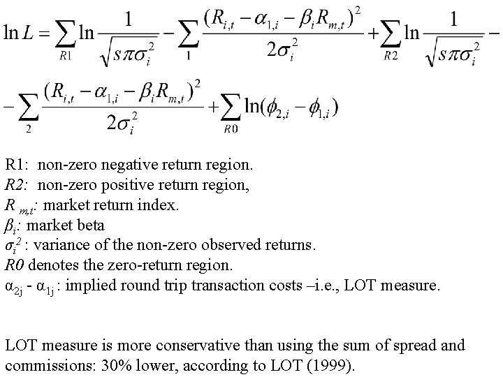
• Lesmond, Ogden, and Trzcinka’s (1999) (LOT) measure LOT use a model-based measure using a Tobin (1958) limited dependent variable (LDV) procedure. Only the time series of daily security returns is needed to estimate the effective transaction costs for a stock. Intuition: Arbitrageurs trade only if the value of accumulated information exceeds the marginal cost of trading. If trading costs are sizable, new information must accumulate longer before investors engage in trading. Therefore, frequency of the zero-return days can be a proxy for the length of information accumulation.

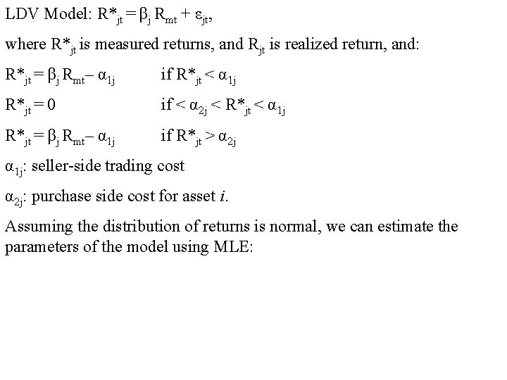
LDV Model: R*jt = βj Rmt + εjt, where R*jt is measured returns, and Rjt is realized return, and: R*jt = βj Rmt– α 1 j if R*jt < α 1 j R*jt = 0 if < α 2 j < R*jt < α 1 j R*jt = βj Rmt– α 1 j if R*jt > α 2 j α 1 j: seller-side trading cost α 2 j: purchase side cost for asset i. Assuming the distribution of returns is normal, we can estimate the parameters of the model using MLE:

R 1: non-zero negative return region. R 2: non-zero positive return region, R m, t: market return index. βi: market beta σi 2 : variance of the non-zero observed returns. R 0 denotes the zero-return region. α 2 j - α 1 j : implied round trip transaction costs –i. e. , LOT measure is more conservative than using the sum of spread and commissions: 30% lower, according to LOT (1999).

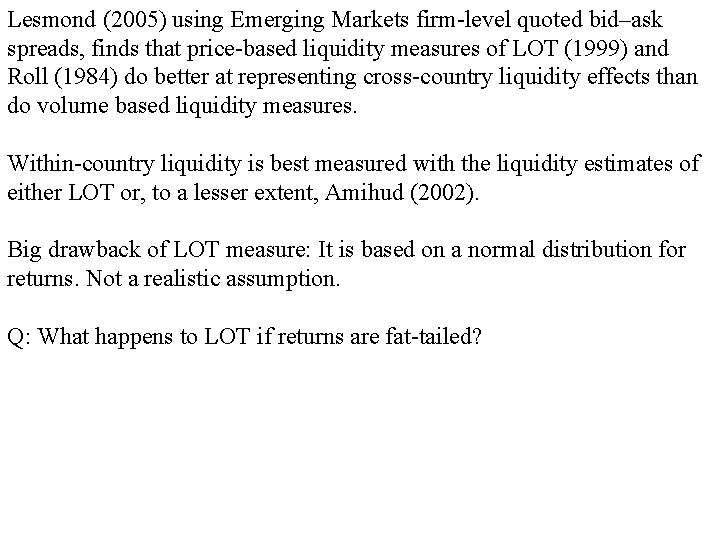
Lesmond (2005) using Emerging Markets firm-level quoted bid–ask spreads, finds that price-based liquidity measures of LOT (1999) and Roll (1984) do better at representing cross-country liquidity effects than do volume based liquidity measures. Within-country liquidity is best measured with the liquidity estimates of either LOT or, to a lesser extent, Amihud (2002). Big drawback of LOT measure: It is based on a normal distribution for returns. Not a realistic assumption. Q: What happens to LOT if returns are fat-tailed?

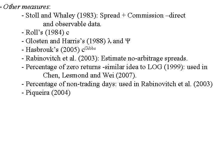
• Other measures: - Stoll and Whaley (1983): Spread + Commission –direct and observable data. - Roll’s (1984) c - Glosten and Harris’s (1988) λ and Ψ - Hasbrouk’s (2005) c. Gibbs - Rabinovitch et al. (2003): Estimate no-arbitrage spreads. - Percentage of zero returns -similar idea to LOG (1999): used in Chen, Lesmond and Wei (2007). - Percentage of non-trading days: used in Rabinovitch et al. (2003) - Piqueira (2004)

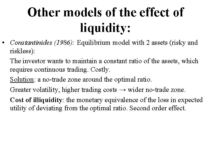
Other models of the effect of liquidity: • Constantinides (1986): Equilibrium model with 2 assets (risky and riskless): The investor wants to maintain a constant ratio of the assets, which requires continuous trading. Costly. Solution: a no-trade zone around the optimal ratio. Greater volatility, higher trading costs → wider no-trade zone. Cost of illiquidity: the monetary equivalence of the loss in expected utility of deviating from the optimal ratio. Second order effect.

• Huang (2003): Equilibrium model with two assets and random liquidity shocks. One liquid, one illiquid. - The net-of-transaction-costs return of the illiquid asset is risky. - Optimal policy: invest in a combination of the two assets for some range of liquidity premium. - Wider range for higher risk aversion, trading costs and prob. of shock arrival. - No borrowing constraint → liquidity premium equals the PV of trading costs, as in the case of fixed horizon (equating net returns). - Borrowing constraint → higher liquidity premium, reflecting the risk. - Older investors are more likely to hold the illiquid asset. - Liquidity premium is higher for smaller relative supply of liquid asset.

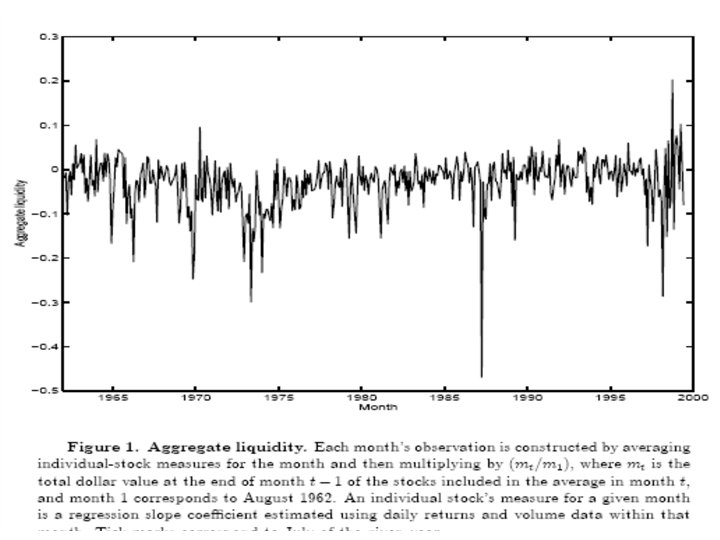
Liquidity risk • Pastor and Stambaugh (2003): Fama-Mac. Beth approach • Greater exposure to liquidity risk → higher expected return. • Liquidity measure γi, t: estimate for each month t using the daily model Rei, d = θi + Φi*Ri, d-1 + γi*sign(Rei, d-1)*Vi, d-1 + ei, d. Rei, d = excess return over Rm, d. V = volume in USD. γi < 0. Reflects return reversal after trading, the liquidity “cost” in terms of return reversal: The larger the volume, the larger the return reversal, the larger the cost. • γ is more negative for more illiquid stocks. The model is estimated each month for each stock (daily data). Market liquidity – gt – is the average across stocks in each month.

gt is autocorrelated. Pastor and Stambaugh (2003) use a 2 -step filter: 1) Δgt = (mt/m 1962) Σi (gi, t - gi, t-1) /Nt , mt = total $ value at the end of month t-1 of stocks included in month t. Nt= number of stocks in month t. 2) Δgt = a + b*Δgt-1 + c*(m t/m 1962)*gγt-1 + Lt. Lt: ”liquidity” innovation The stock’s exposure to market liquidity is measured by βLi : Ri, t = β 0 i + βLi *Lt + βMi *RMt + βS *SMBt + βHi*HMLt + ei, t. βLi is positively correlated with size, negatively with βM, βS and βH (weak for all). Stocks are sorted into 10 portfolios by their βLi. Findings: α’s from market or FF models are strongly increasing in βLi

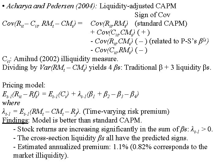
• Acharya and Pedersen (2004): Liquidity-adjusted CAPM Sign of Cov(Rit – Cit, RMt – CMt) = Cov(Rit, RMt) (standard CAPM) + Cov(Cit, CMt) ( + ) - Cov(Rit, CMt) ( – ) (related to P-S’s βLi) - Cov(Cit, RMt) ( – ) Cit: Amihud (2002) illiquidity measure. Dividing by Var(RMt – CMt) yields 4 βs: Traditional β + 3 liquidity βs. Pricing model: Et-1(Rit – Rft) = Et-1(Ci) + λt-1(β 1 + β 2 – β 3 – β 4) where λt-1 = Et-1(RMt – CMt – Rf). (Time-varying risk premium) Findings: Model is better than standard CAPM. - Stock returns are increasing significantly in the sum of βs: λt-1 > 0. - The cross-section liquidity βs all have the predicted signs. - Estimated annualized premium: 1. 1% (0. 82% corresponds to the market illiquidity).

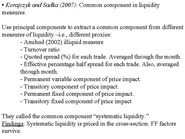
• Korajczyk and Sadka (2007): Common component in liquidity measures. Use principal components to extract a common component from different measures of liquidity –i. e. , different proxies: - Amihud (2002) illiquid measure - Turnover ratio - Quoted spread (%) for each trade. Averaged through the month. - Effective percentage half spread for each trade. Also, averaged through month. - Permanent variable component of price impact. - Transitory component of price impact. - Permanent fixed component of price impact. - Transitory fixed component of price impact They called the common component “systematic liquidity. ” Findings: Systematic liquidity is priced in the cross-section. FF factors survive.

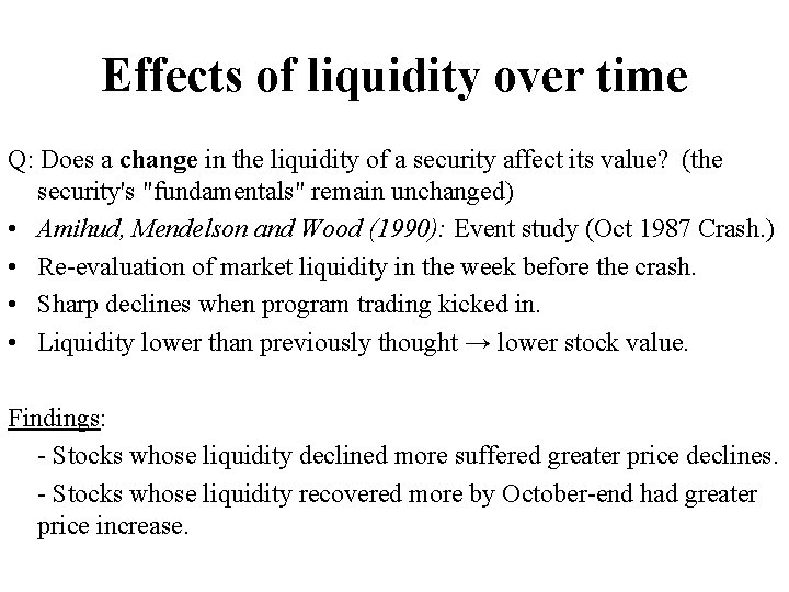
Effects of liquidity over time Q: Does a change in the liquidity of a security affect its value? (the security's "fundamentals" remain unchanged) • Amihud, Mendelson and Wood (1990): Event study (Oct 1987 Crash. ) • Re-evaluation of market liquidity in the week before the crash. • Sharp declines when program trading kicked in. • Liquidity lower than previously thought → lower stock value. Findings: - Stocks whose liquidity declined more suffered greater price declines. - Stocks whose liquidity recovered more by October-end had greater price increase.

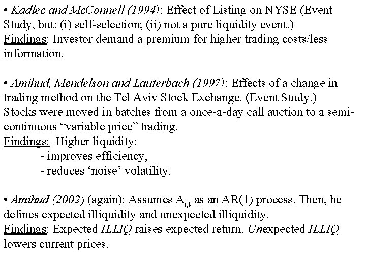
• Kadlec and Mc. Connell (1994): Effect of Listing on NYSE (Event Study, but: (i) self-selection; (ii) not a pure liquidity event. ) Findings: Investor demand a premium for higher trading costs/less information. • Amihud, Mendelson and Lauterbach (1997): Effects of a change in trading method on the Tel Aviv Stock Exchange. (Event Study. ) Stocks were moved in batches from a once-a-day call auction to a semicontinuous “variable price” trading. Findings: Higher liquidity: - improves efficiency, - reduces ‘noise’ volatility. • Amihud (2002) (again): Assumes Ai, t as an AR(1) process. Then, he defines expected illiquidity and unexpected illiquidity. Findings: Expected ILLIQ raises expected return. Unexpected ILLIQ lowers current prices.