Lecture 4 Uninformed Search Vikas Ashok Department of

Lecture 4 Uninformed Search Vikas Ashok Department of Computer Science ODU Reading for Next Class: Chapter 3, Russell and Norvig Artificial Intelligence Special thanks for Dr. Yaohang Li for sharing the slides

Review • Last Class – Problem Solving Agent • Goal Formulation • Problem Formulation • This Class – Uninformed Search Algorithms • Breadth-first search • Depth-first search – Analysis • Time Complexity • Space Complexity • Other Measures • Next Class – Informed Search Algorithms Artificial Intelligence

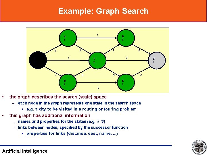
Example: Graph Search 1 A 4 1 1 1 5 S 3 1 D 3 3 2 C 2 3 3 B 2 G 0 4 E 1 2 • the graph describes the search (state) space – each node in the graph represents one state in the search space • e. g. a city to be visited in a routing or touring problem • this graph has additional information – names and properties for the states (e. g. S, 3) – links between nodes, specified by the successor function • properties for links (distance, cost, name, . . . ) Artificial Intelligence

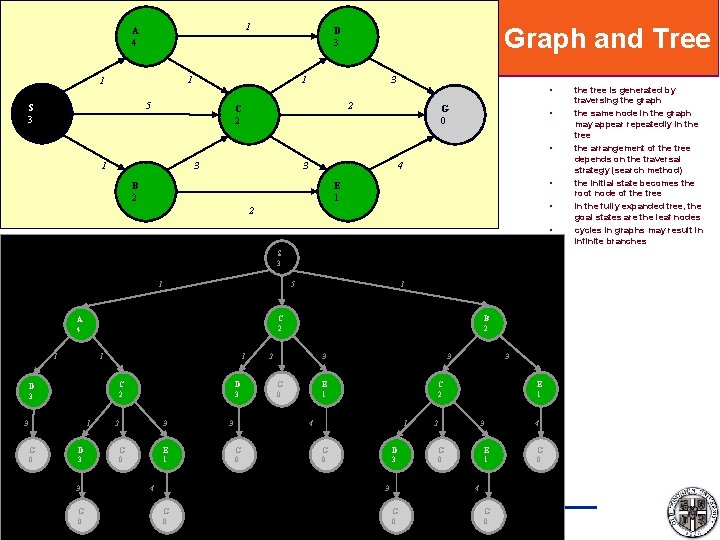
1 A 4 1 1 1 5 S 3 Graph and Tree D 3 3 • 2 C 2 G 0 • • 1 3 3 4 B 2 • E 1 • 2 • S 3 1 C 2 A 4 1 1 1 G 0 1 C 2 D 3 3 G 0 1 5 D 3 2 3 G 0 E 1 4 3 B 2 2 3 G 0 3 E 1 C 2 4 G 0 1 G 0 D 3 3 G 0 Artificial Intelligence 3 4 3 2 G 0 E 1 4 G 0 the tree is generated by traversing the graph the same node in the graph may appear repeatedly in the tree the arrangement of the tree depends on the traversal strategy (search method) the initial state becomes the root node of the tree in the fully expanded tree, the goal states are the leaf nodes cycles in graphs may result in infinite branches

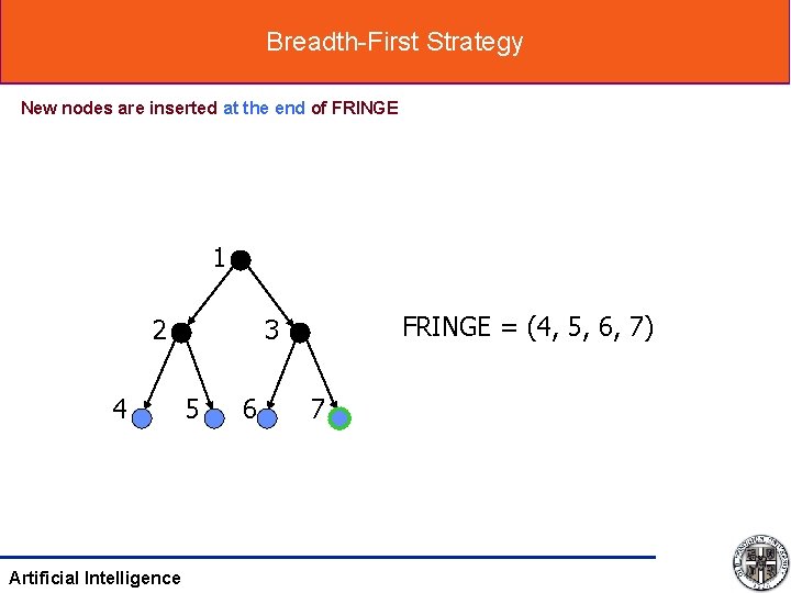
Implementation of Breadth-first Search • Fringe – Queue (FIFO) – Put all newly generated successors at the end of the queue • Shallow nodes are expanded before deeper nodes Artificial Intelligence

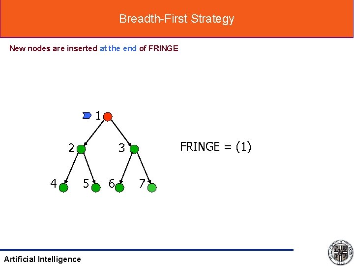
Breadth-First Strategy New nodes are inserted at the end of FRINGE 1 2 4 Artificial Intelligence FRINGE = (1) 3 5 6 7

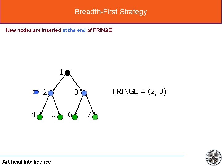
Breadth-First Strategy New nodes are inserted at the end of FRINGE 1 2 4 Artificial Intelligence FRINGE = (2, 3) 3 5 6 7

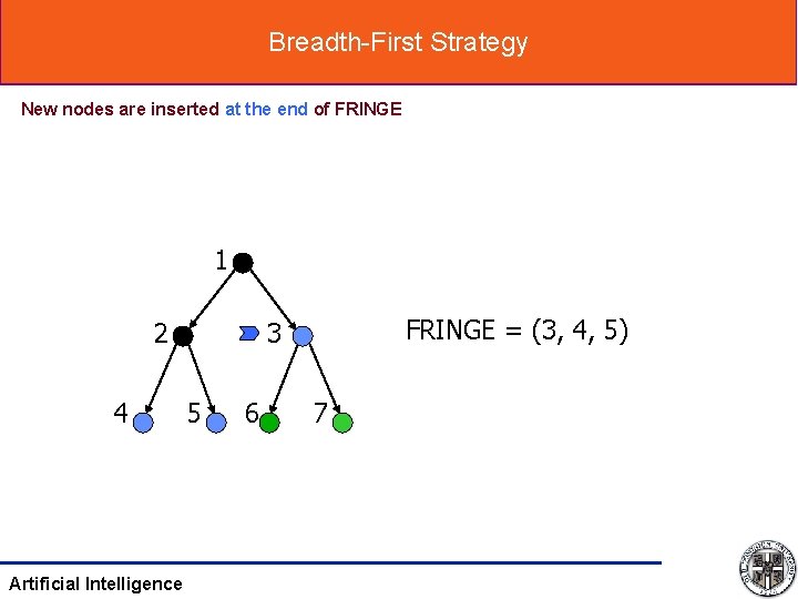
Breadth-First Strategy New nodes are inserted at the end of FRINGE 1 2 4 Artificial Intelligence FRINGE = (3, 4, 5) 3 5 6 7

Breadth-First Strategy New nodes are inserted at the end of FRINGE 1 2 4 Artificial Intelligence FRINGE = (4, 5, 6, 7) 3 5 6 7

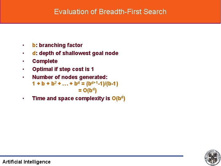
Evaluation of Breadth-First Search • • • b: branching factor d: depth of shallowest goal node Complete Optimal if step cost is 1 Number of nodes generated: 1 + b 2 + … + bd = (bd+1 -1)/(b-1) = O(bd) Time and space complexity is O(bd) Artificial Intelligence

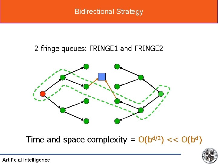
Bidirectional Search • Run two simultaneous searches – One forward from the initial sate – The other backward from the goal – Stopping when the two searches meet in the middle • Implementation – Keep two fringes – Compare two fringes at every steps – When the intersection is not empty, the search stops • Analysis – Optimality • Yes – Complete • Yes Artificial Intelligence

Bidirectional Strategy 2 fringe queues: FRINGE 1 and FRINGE 2 Time and space complexity = O(bd/2) << O(bd) Artificial Intelligence

Implementation of Depth-first Search • Fringe – Stack (LIFO) – Push all newly generated successors into the stack Artificial Intelligence

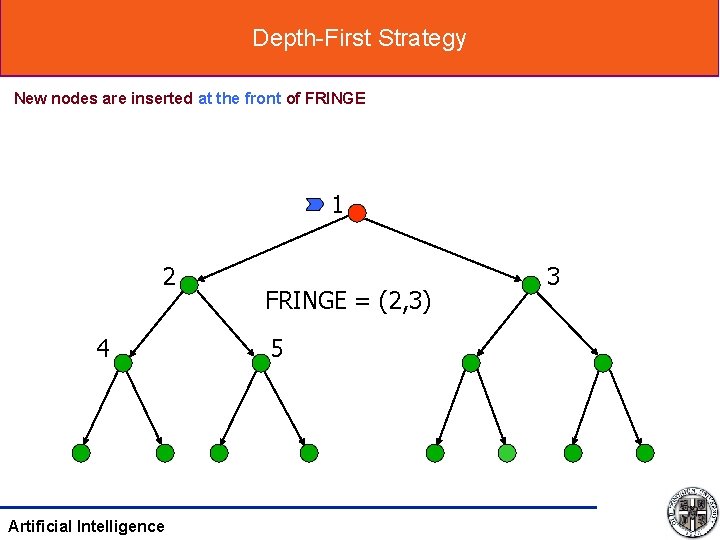
Depth-First Strategy New nodes are inserted at the front of FRINGE 1 2 4 Artificial Intelligence FRINGE = (2, 3) 5 3

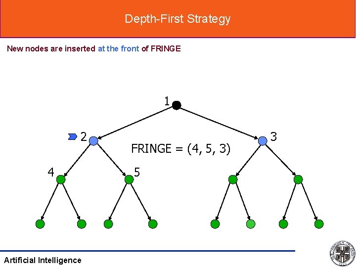
Depth-First Strategy New nodes are inserted at the front of FRINGE 1 2 4 Artificial Intelligence FRINGE = (4, 5, 3) 5 3

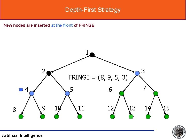
Depth-First Strategy New nodes are inserted at the front of FRINGE 1 2 FRINGE = (8, 9, 5, 3) 4 8 5 9 Artificial Intelligence 3 10 7 6 11 12 13 14 15

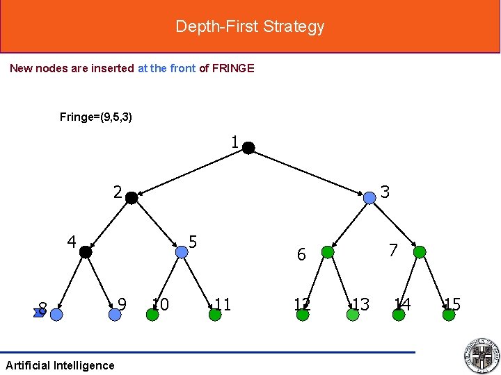
Depth-First Strategy New nodes are inserted at the front of FRINGE Fringe=(9, 5, 3) 1 2 3 4 8 Artificial Intelligence 5 9 10 7 6 11 12 13 14 15

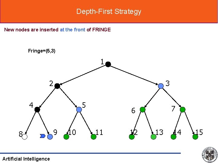
Depth-First Strategy New nodes are inserted at the front of FRINGE Fringe=(5, 3) 1 2 3 4 8 Artificial Intelligence 5 9 10 7 6 11 12 13 14 15

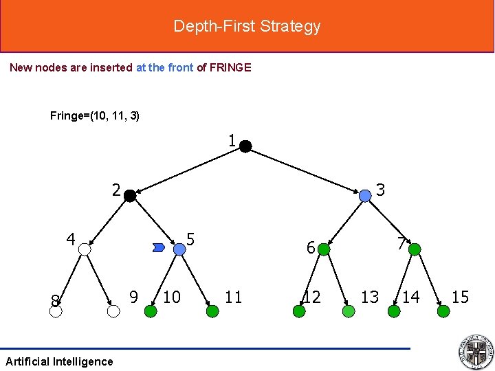
Depth-First Strategy New nodes are inserted at the front of FRINGE Fringe=(10, 11, 3) 1 2 3 4 8 Artificial Intelligence 5 9 10 7 6 11 12 13 14 15

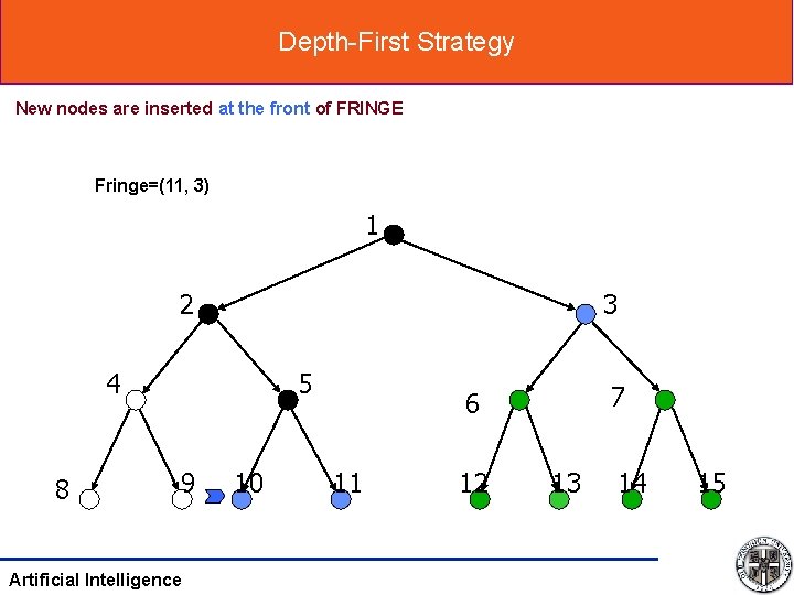
Depth-First Strategy New nodes are inserted at the front of FRINGE Fringe=(11, 3) 1 2 3 4 8 5 9 Artificial Intelligence 10 7 6 11 12 13 14 15

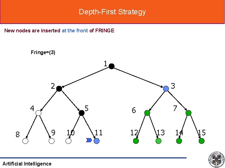
Depth-First Strategy New nodes are inserted at the front of FRINGE Fringe=(3) 1 2 3 4 8 5 9 Artificial Intelligence 10 7 6 11 12 13 14 15

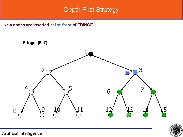
Depth-First Strategy New nodes are inserted at the front of FRINGE Fringe=(6, 7) 1 2 3 4 8 5 9 Artificial Intelligence 10 7 6 11 12 13 14 15

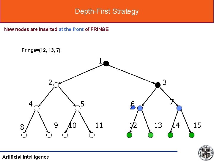
Depth-First Strategy New nodes are inserted at the front of FRINGE Fringe=(12, 13, 7) 1 2 3 4 8 Artificial Intelligence 5 9 10 7 6 11 12 13 14 15

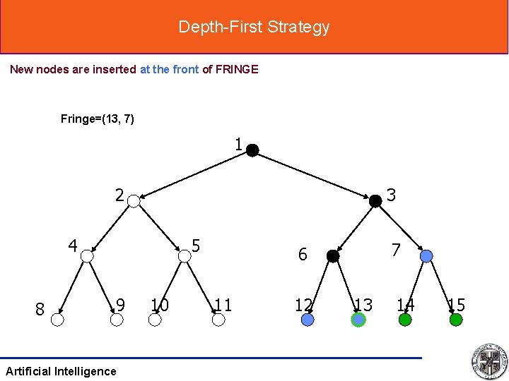
Depth-First Strategy New nodes are inserted at the front of FRINGE Fringe=(13, 7) 1 2 3 4 8 5 9 Artificial Intelligence 10 7 6 11 12 13 14 15

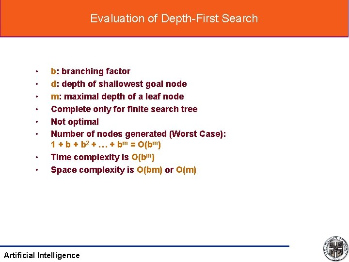
Evaluation of Depth-First Search • • b: branching factor d: depth of shallowest goal node m: maximal depth of a leaf node Complete only for finite search tree Not optimal Number of nodes generated (Worst Case): 1 + b 2 + … + bm = O(bm) Time complexity is O(bm) Space complexity is O(bm) or O(m) Artificial Intelligence

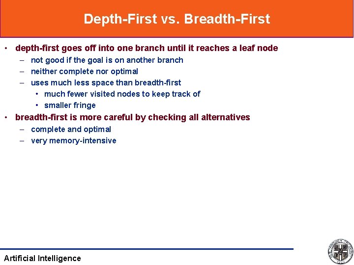
Depth-First vs. Breadth-First • depth-first goes off into one branch until it reaches a leaf node – not good if the goal is on another branch – neither complete nor optimal – uses much less space than breadth-first • much fewer visited nodes to keep track of • smaller fringe • breadth-first is more careful by checking all alternatives – complete and optimal – very memory-intensive Artificial Intelligence

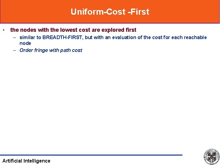
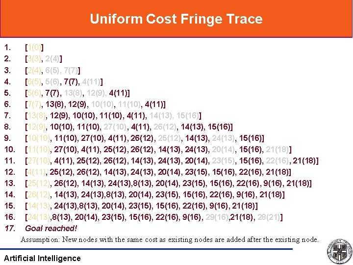
Uniform-Cost -First • the nodes with the lowest cost are explored first – similar to BREADTH-FIRST, but with an evaluation of the cost for each reachable node – Order fringe with path cost Artificial Intelligence

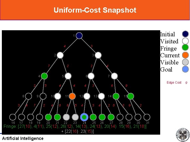
Uniform-Cost Snapshot Initial Visited Fringe Current Visible Goal 1 4 3 2 3 7 2 4 5 2 8 3 16 17 5 9 4 7 18 2 2 19 4 20 6 4 10 4 11 8 21 4 6 22 4 12 5 23 4 24 7 3 6 13 3 25 14 4 26 2 8 27 Edge Cost 9 15 3 28 9 29 2 30 31 Fringe: [27(10), 4(11), 25(12), 26(12), 14(13), 20(14), 15(16), 21(18)] + [22(16), 23(15)] Artificial Intelligence 9

Uniform Cost Fringe Trace 1. 2. 3. 4. 5. 6. 7. 8. 9. 10. 11. 12. 13. 14. 15. 16. 17. [1(0)] [3(3), 2(4)] [2(4), 6(5), 7(7)] [6(5), 5(6), 7(7), 4(11)] [5(6), 7(7), 13(8), 12(9), 4(11)] [7(7), 13(8), 12(9), 10(10), 11(10), 4(11)] [13(8), 12(9), 10(10), 11(10), 4(11), 14(13), 15(16)] [12(9), 10(10), 11(10), 27(10), 4(11), 26(12), 14(13), 15(16)] [10(10), 11(10), 27(10), 4(11), 26(12), 25(12), 14(13), 24(13), 15(16)] [11(10), 27(10), 4(11), 25(12), 26(12), 14(13), 20(14), 15(16), 21(18)] [27(10), 4(11), 25(12), 26(12), 14(13), 24(13), 20(14), 23(15), 15(16), 22(16), 21(18)] [25(12), 26(12), 14(13), 24(13), 8(13), 20(14), 23(15), 15(16), 22(16), 9(16), 21(18)] [14(13), 24(13), 8(13), 20(14), 23(15), 15(16), 22(16), 9(16), 21(18)] [24(13), 8(13), 20(14), 23(15), 15(16), 22(16), 9(16), 21(18), 28(21)] Goal reached! Assumption: New nodes with the same cost as existing nodes are added after the existing node. Artificial Intelligence

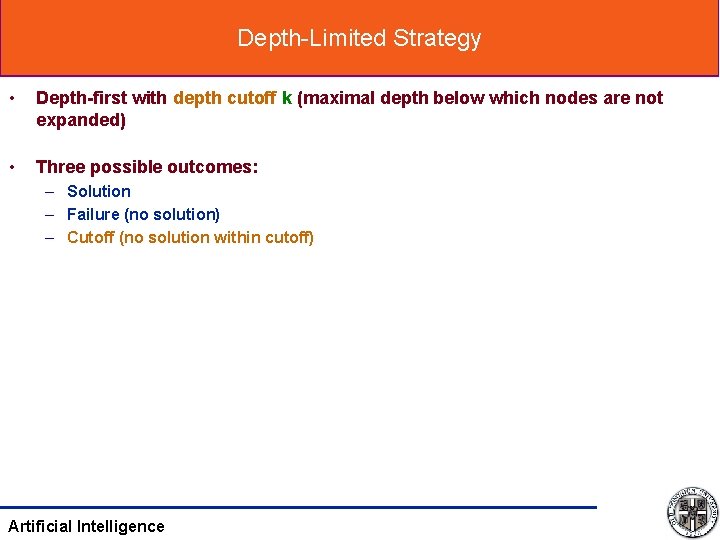
Depth-Limited Strategy • Depth-first with depth cutoff k (maximal depth below which nodes are not expanded) • Three possible outcomes: – Solution – Failure (no solution) – Cutoff (no solution within cutoff) Artificial Intelligence

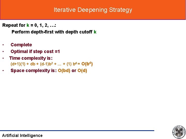
Iterative Deepening Strategy Repeat for k = 0, 1, 2, …: Perform depth-first with depth cutoff k • • • Complete Optimal if step cost =1 Time complexity is: (d+1)(1) + db + (d-1)b 2 + … + (1) bd = O(bd) • Space complexity is: O(bd) or O(d) Artificial Intelligence

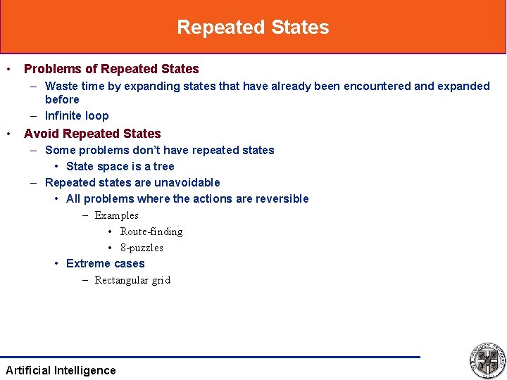
Repeated States • Problems of Repeated States – Waste time by expanding states that have already been encountered and expanded before – Infinite loop • Avoid Repeated States – Some problems don’t have repeated states • State space is a tree – Repeated states are unavoidable • All problems where the actions are reversible – Examples • Route-finding • 8 -puzzles • Extreme cases – Rectangular grid Artificial Intelligence

Avoid Repeated States in DFS • Problems in Depth-first Search – May lead to infinite loop • Cannot find a solution • Depth-first Search – Keep track of the path from the root to the current node – Compare the current node with the nodes in the path • Discard it if it is already in the path – Prevent infinite loop Artificial Intelligence

Eliminate Repeated Nodes • Closed List – Store every expanded node • Open List (Fringe) – Store unexpanded nodes • Graph-Search – Match current node with nodes in Closed List – Discard if it is in closed list • Tree-Search – Search for the search tree instead of the state space – Without the data structure of closed list • Discussion – Time/Space Trade-off Artificial Intelligence

Node Information in Search Tree • • State: The state in the state space to which the node corresponds Parent: The node in the search tree that generated this node Action: The action that was applied to the parent to generate the node Path Cost: The path cost from the initial state to the node Artificial Intelligence

Pseudocode for Depth First Search Declare two empty lists: Open and Closed. Add Start node to our Open list. While our Open list is not empty, loop the following: Remove the first node from our Open List. Check to see if the removed node is our destination. If the removed node is our destination, break out of the loop, add the node to our Closed list, and return the value of our Closed list. If the removed node is not our destination, continue the loop. Extract the neighbors of our above removed node. Add the neighbors to the beginning of our Open list, and add the removed node to our Closed list. Continue looping. Artificial Intelligence

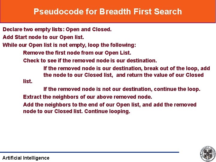
Pseudocode for Breadth First Search Declare two empty lists: Open and Closed. Add Start node to our Open list. While our Open list is not empty, loop the following: Remove the first node from our Open List. Check to see if the removed node is our destination. If the removed node is our destination, break out of the loop, add the node to our Closed list, and return the value of our Closed list. If the removed node is not our destination, continue the loop. Extract the neighbors of our above removed node. Add the neighbors to the end of our Open list, and add the removed node to our Closed list. Continue looping. Artificial Intelligence

Summary • Breadth-first search – Analysis • Depth-first search – Analysis • • • Uniform-cost search Depth-limited search (Optional) Iterative deepening search (Optional) Artificial Intelligence

What I want you to do • Review Chapter 3 Artificial Intelligence