Last Time Microfacet models Diffuse OrenNayar Specular TorranceSparrow

Last Time • Microfacet models – Diffuse • Oren-Nayar – Specular • Torrance-Sparrow – Blinn – Ashikhmin-Shirley – Ward – Schlick • Lafortune’s model • Glossy over Diffuse 02/4/05 © 2005 University of Wisconsin

Today • • Assignment 1, Part 2, h=4 More reflectance models Materials Textures 02/4/05 © 2005 University of Wisconsin

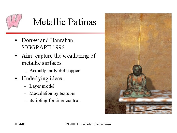
Metallic Patinas • Dorsey and Hanrahan, SIGGRAPH 1996 • Aim: capture the weathering of metallic surfaces – Actually, only did copper • Underlying ideas: – Layer model – Modulation by textures – Scripting for time control 02/4/05 © 2005 University of Wisconsin

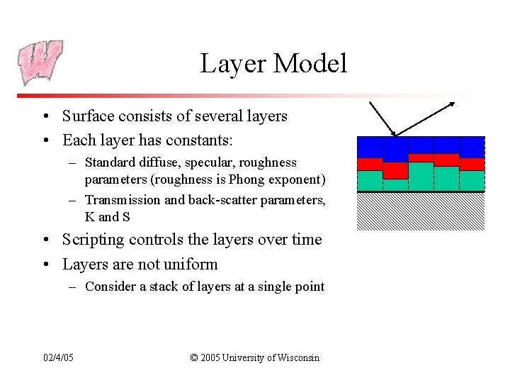
Layer Model • Surface consists of several layers • Each layer has constants: – Standard diffuse, specular, roughness parameters (roughness is Phong exponent) – Transmission and back-scatter parameters, K and S • Scripting controls the layers over time • Layers are not uniform – Consider a stack of layers at a single point 02/4/05 © 2005 University of Wisconsin

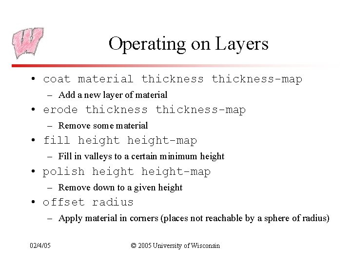
Operating on Layers • coat material thickness-map – Add a new layer of material • erode thickness-map – Remove some material • fill height-map – Fill in valleys to a certain minimum height • polish height-map – Remove down to a given height • offset radius – Apply material in corners (places not reachable by a sphere of radius) 02/4/05 © 2005 University of Wisconsin

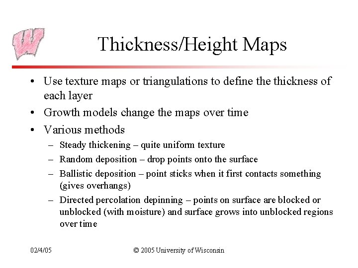
Thickness/Height Maps • Use texture maps or triangulations to define thickness of each layer • Growth models change the maps over time • Various methods – Steady thickening – quite uniform texture – Random deposition – drop points onto the surface – Ballistic deposition – point sticks when it first contacts something (gives overhangs) – Directed percolation depinning – points on surface are blocked or unblocked (with moisture) and surface grows into unblocked regions over time 02/4/05 © 2005 University of Wisconsin

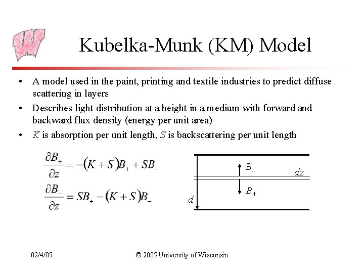
Kubelka-Munk (KM) Model • A model used in the paint, printing and textile industries to predict diffuse scattering in layers • Describes light distribution at a height in a medium with forward and backward flux density (energy per unit area) • K is absorption per unit length, S is backscattering per unit length Bd 02/4/05 © 2005 University of Wisconsin B+ dz

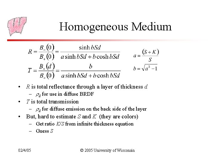
Homogeneous Medium • R is total reflectance through a layer of thickness d – d for use in diffuse BRDF • T is total transmission – d for diffuse emission on the back side of the layer • But, hard to estimate S and K (they are colors) – Get ratio K/S from infinite thickness equation – Guess S 02/4/05 © 2005 University of Wisconsin

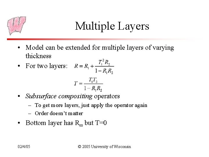
Multiple Layers • Model can be extended for multiple layers of varying thickness • For two layers: • Subsurface compositing operators – To get more layers, just apply the operator again – Order doesn’t matter • Bottom layer has R but T=0 02/4/05 © 2005 University of Wisconsin

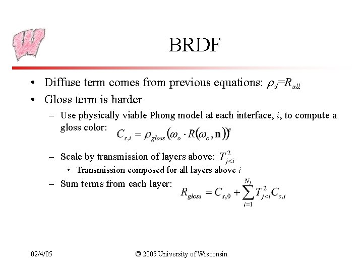
BRDF • Diffuse term comes from previous equations: d=Rall • Gloss term is harder – Use physically viable Phong model at each interface, i, to compute a gloss color: – Scale by transmission of layers above: • Transmission composed for all layers above i – Sum terms from each layer: 02/4/05 © 2005 University of Wisconsin

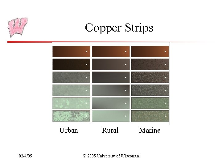
Copper Strips Urban 02/4/05 Rural © 2005 University of Wisconsin Marine

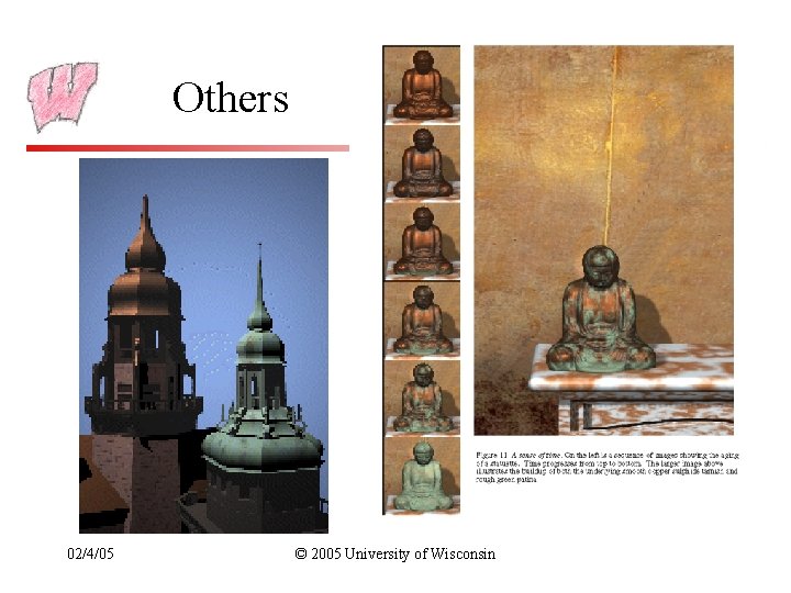
Others 02/4/05 © 2005 University of Wisconsin

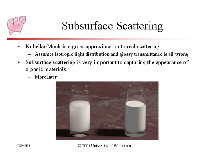
Subsurface Scattering • Kubelka-Munk is a gross approximation to real scattering – Assumes isotropic light distribution and glossy transmittance is all wrong • Subsurface scattering is very important to capturing the appearance of organic materials – More later 02/4/05 © 2005 University of Wisconsin

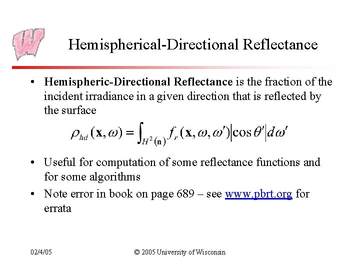
Hemispherical-Directional Reflectance • Hemispheric-Directional Reflectance is the fraction of the incident irradiance in a given direction that is reflected by the surface • Useful for computation of some reflectance functions and for some algorithms • Note error in book on page 689 – see www. pbrt. org for errata 02/4/05 © 2005 University of Wisconsin

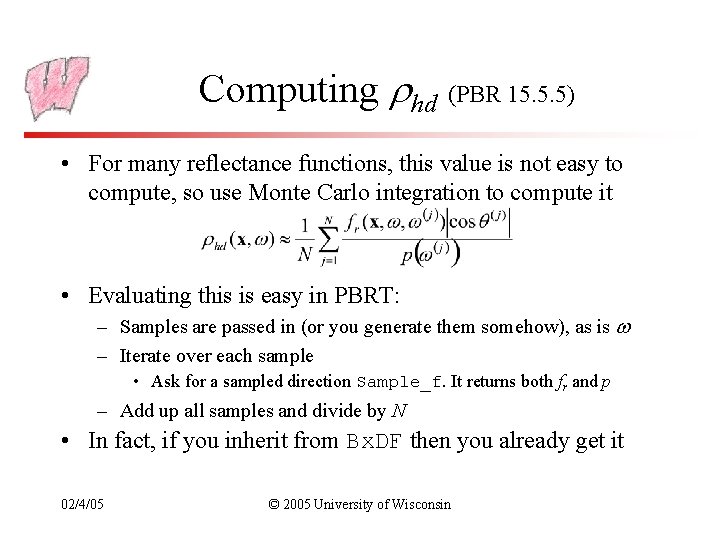
Computing hd (PBR 15. 5. 5) • For many reflectance functions, this value is not easy to compute, so use Monte Carlo integration to compute it • Evaluating this is easy in PBRT: – Samples are passed in (or you generate them somehow), as is – Iterate over each sample • Ask for a sampled direction Sample_f. It returns both fr and p – Add up all samples and divide by N • In fact, if you inherit from Bx. DF then you already get it 02/4/05 © 2005 University of Wisconsin

PBRT BSDF Structures (PBR Sect 10. 1) • A Bx. DF is a component of a BSDF – one of the things we have been looking at so far • BSDF can be made up of multiple components • The PBRT BSDF structure has code for managing these components – read Chapter 10 • When sampling, choose a Bx. DF – Uniform probability of choosing any one matching component – PDF of choosing some direction must account for all components • But it still assumes we’re talking about a single point 02/4/05 © 2005 University of Wisconsin

PBRT Materials (PBR Sect 10. 2) • A Material described how the BSDF varies over the entire surface of an object • All parameters to the components Bx. DFs are given in the form of textures – More on textures in a minute • The job of the Material is: – Manage local surface variations via textures and pass a single set of point properties (color, normal, etc) to BSDFs – Provide BSDFs with information about the neighborhood, particularly the geometric normal and the shading normal (bump mapped or otherwise modified) 02/4/05 © 2005 University of Wisconsin

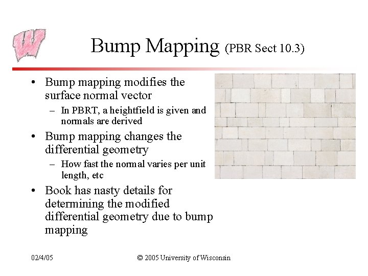
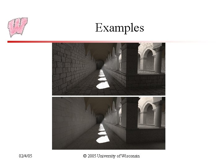
Bump Mapping (PBR Sect 10. 3) • Bump mapping modifies the surface normal vector – In PBRT, a heightfield is given and normals are derived • Bump mapping changes the differential geometry – How fast the normal varies per unit length, etc • Book has nasty details for determining the modified differential geometry due to bump mapping 02/4/05 © 2005 University of Wisconsin

Examples 02/4/05 © 2005 University of Wisconsin

Textures (PBR Chap 11) • Read Chapter 11 for functionality (but not details) • Highlights: – Sampling and Aliasing – how to compute rate of change of surface u, v parameters with respect to image coordinates x, y • Needed for texture filtering – Generating texture coordinates – Various forms of textures • Texture maps (images) • Procedural textures of various forms 02/4/05 © 2005 University of Wisconsin

Texture Coordinates • On the surface, we have u, v coordinates, defined as part of the shape definition – Sphere? Cylinder? • For texturing, we need s, t coordinates – not the same • There are various mappings that take (x, y, z) and convert to (s, t) – Actually, take entire differential geometry, such as normal vector and dp/du and dp/dv 02/4/05 © 2005 University of Wisconsin

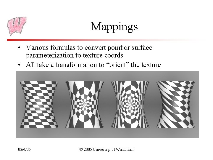
Mappings • Various formulas to convert point or surface parameterization to texture coords • All take a transformation to “orient” the texture 02/4/05 © 2005 University of Wisconsin

Texture Types • Constant value, Scale: t 1 * t 2, Mix: (1 -a)*t 1+a*t 2 – Use these for texture blends • Bilinear: Bilinearly interpolate from four constant values – What type of shading interpolation does this perform? • Images – Lots of details about caching and mipmapping – ignore them • Procedural textures: – Program computes values – each texture must be a separate class • Perlin noise – Core functionality 02/4/05 © 2005 University of Wisconsin

Texture Antialiasing • If you define a new procedural texture, you should correctly anti-alias it • Information about ds/dx, dt/dx, ds/dy, dt/dy is available – Tells you how fast texture coordinates change on screen, which tells you how many “texels” appear in one pixel • There are many examples in the book of how this might be done, but as a fallback you can always super-sample the texture function 02/4/05 © 2005 University of Wisconsin

Next Time • Light Sources • Direct Lighting 02/4/05 © 2005 University of Wisconsin