IPAM Workshop on Image Processing for Random Shapes

IPAM Workshop on Image Processing for Random Shapes: Applications to Brain Mapping, Geophysics and Astrophysics UCLA May 21 -25, 2007 Geometric Shape Descriptors for Shape Analysis and Sulcal Classification of MRI Data Monica K. Hurdal Department of Mathematics, Florida State University, Tallahassee mhurdal@math. fsu. edu http: //www. math. fsu. edu/~mhurdal

Motivation • Increasingly, diseases that affect brain function are being correlated to structural brain changes. • Classification and identification of differences in brain anatomy (i. e. differences in shape) due to disease is difficult due to individual variability in folding patterns. • Parcellation and labeling of cortical features are critical for brain cartography and conveying information to compare subjects or populations. • Parcellation and labeling are manually intensive processes confounded by variability in folding patterns. • Methods are needed to quantify properties of the shape of the cortical surface on a global as well as local level.

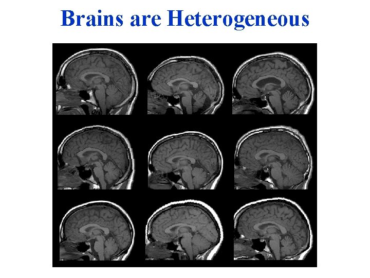
Brains are Heterogeneous Slide from Duke course

Important Questions • How much variation is there in the size, shape or location of an individual healthy brain structure? • To what extend does function and disease depend on the anatomy of the brain? • Potential of using structural abnormality as a measure of development, normal aging, and disease

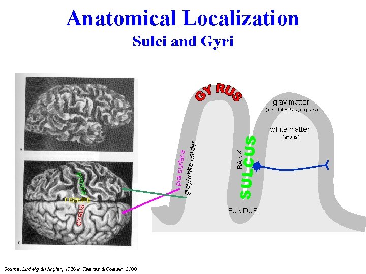
Anatomical Localization Sulci and Gyri gray matter (dendrites & synapses) GYRU S Source: Ludwig & Klingler, 1956 in Tamraz & Comair, 2000 BANK SULCUS FISSURE pial surfa ce gray/whit e border US SULC white matter FUNDUS (axons)

Shape Analysis, Curve Shape Descriptors & Features • Properties of shape curves and surfaces in 3 D can be described by invariant features. • Sulcal or gyral curves that fall in the same class exhibit geometric resemblance, but significant intra-class variations have been observed as well. • Thus, starting with a collection of shape descriptors, it is essential to develop algorithmic procedures to extract (learn) the features that can be used effectively for parcellation, labeling and disease quantification.

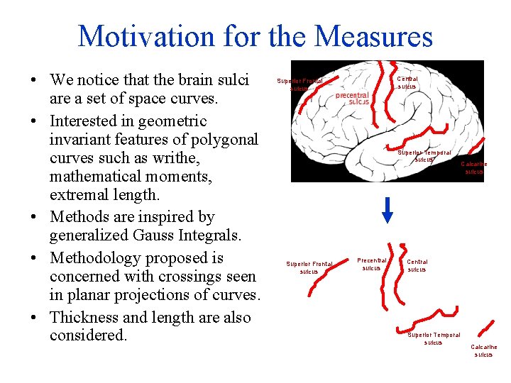
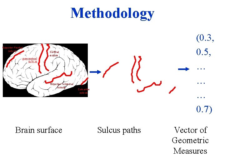
Motivation for the Measures • We notice that the brain sulci are a set of space curves. • Interested in geometric invariant features of polygonal curves such as writhe, mathematical moments, extremal length. • Methods are inspired by generalized Gauss Integrals. • Methodology proposed is concerned with crossings seen in planar projections of curves. • Thickness and length are also considered. Central sulcus Superior Frontal sulcus Superior Temporal sulcus Superior Frontal sulcus Precentral sulcus Calcarine sulcus Central sulcus Superior Temporal sulcus Calcarine sulcus

Geometric Shape Descriptors • Generalized Gauss Integrals • Thickness and Ropelength

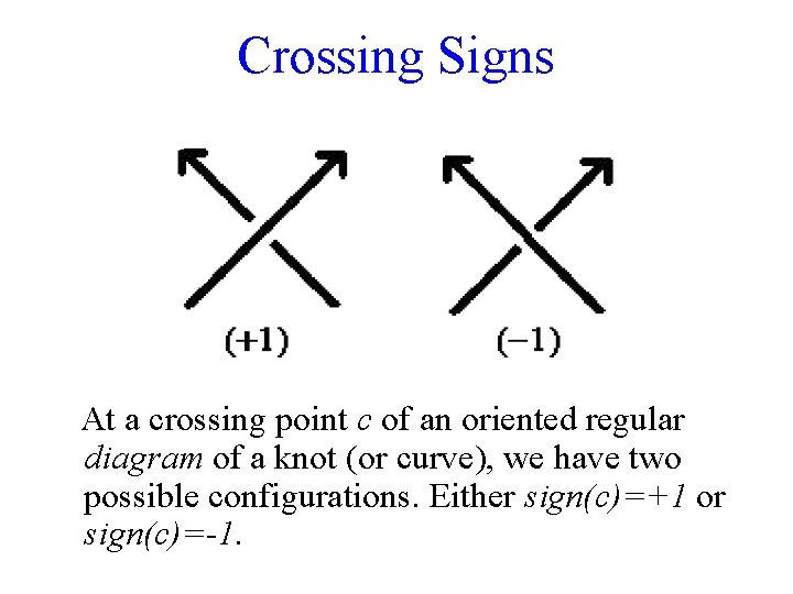
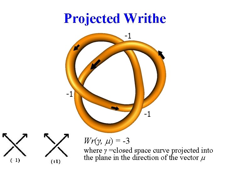
Crossing Signs At a crossing point c of an oriented regular diagram of a knot (or curve), we have two possible configurations. Either sign(c)=+1 or sign(c)=-1.

Projected Writhe -1 -1 -1 Wr(γ, m) = -3 where γ =closed space curve projected into the plane in the direction of the vector m

Writhing Number In general, almost all projections of a curve into the plane in the direction of the vector m will be regular, where at most two projected edges intersect, and that intersection is transverse. For any regular projection, each crossing c can be assigned a value of according to the right hand rule. The Writhe (or projected writhing number), Wr(g), is defined as the average over all projections of the projected writhing number The projected writhing number of a closed space curve γ, denoted by Wr(γ), can be calculated using generalized Gauss integrals.

Calculating Writhe using a Gauss Integral Given a simple closed curve the double integral: , the writhe is defined by where D is the diagonal of • What about polygonal curves? .

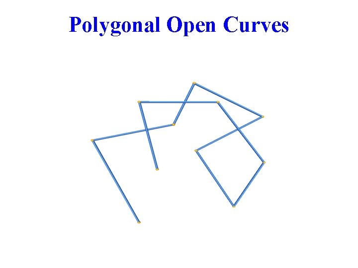
Polygonal Open Curves Source: Knotplot by R Scharein

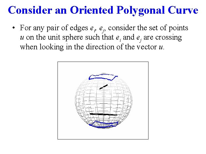
Consider an Oriented Polygonal Curve • For any pair of edges ei, ej, consider the set of points u on the unit sphere such that ei and ej are crossing when looking in the direction of the vector u.

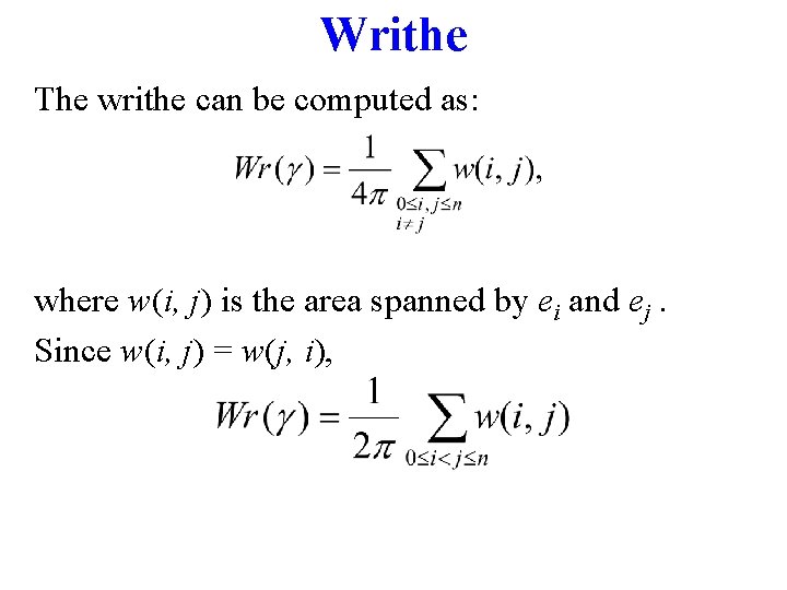
Writhe The writhe can be computed as: where w(i, j) is the area spanned by ei and ej. Since w(i, j) = w(j, i),

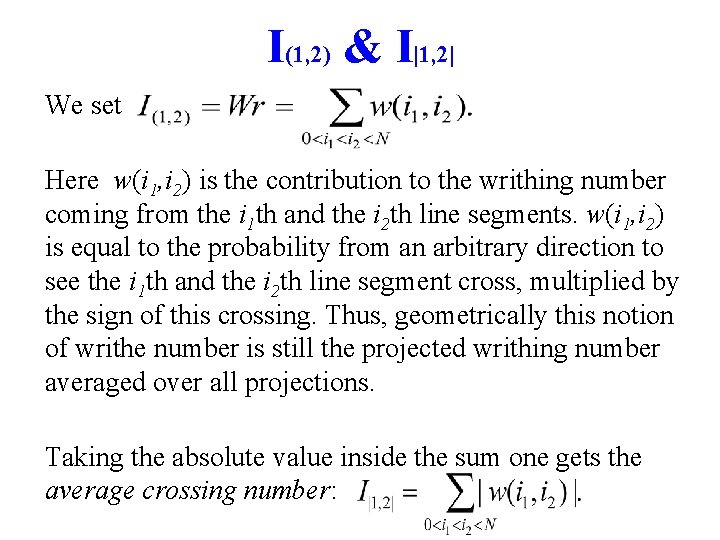
I(1, 2) & I|1, 2| We set Here w(i 1, i 2) is the contribution to the writhing number coming from the i 1 th and the i 2 th line segments. w(i 1, i 2) is equal to the probability from an arbitrary direction to see the i 1 th and the i 2 th line segment cross, multiplied by the sign of this crossing. Thus, geometrically this notion of writhe number is still the projected writhing number averaged over all projections. Taking the absolute value inside the sum one gets the average crossing number:

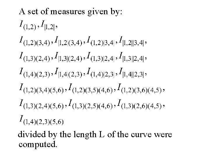
Higher Order Writhing Numbers: A Family of Measures By combining these numbers, we can make a whole set of structural higher order writhing measures, e. g. where N is the number of vertices for the polygonal curve Reference: P. Rogen, B. Fain; 2003 PNAS, Vol 100 No. 1, 119 -124

Importance • Plane curves A and B possess the same writhe and average crossing number. • The higher-order invariants, however, distinguish the two curves. Reference: P. Rogen, B. Fain; 2003 PNAS, Vol 100 No. 1, 119 -124

A set of measures given by: divided by the length L of the curve were computed.

Geometric Shape Descriptors • Generalized Gauss Integrals • Thickness and Ropelength

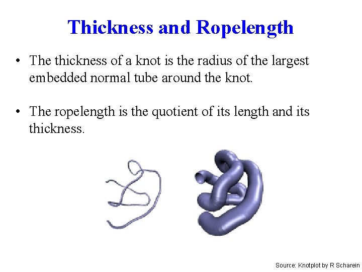
Thickness and Ropelength • The thickness of a knot is the radius of the largest embedded normal tube around the knot. • The ropelength is the quotient of its length and its thickness. Source: Knotplot by R Scharein

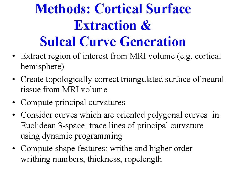
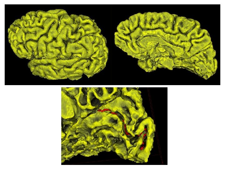
Methods: Cortical Surface Extraction & Sulcal Curve Generation • Extract region of interest from MRI volume (e. g. cortical hemisphere) • Create topologically correct triangulated surface of neural tissue from MRI volume • Compute principal curvatures • Consider curves which are oriented polygonal curves in Euclidean 3 -space: trace lines of principal curvature using dynamic programming • Compute shape features: writhe and higher order writhing numbers, thickness, ropelength

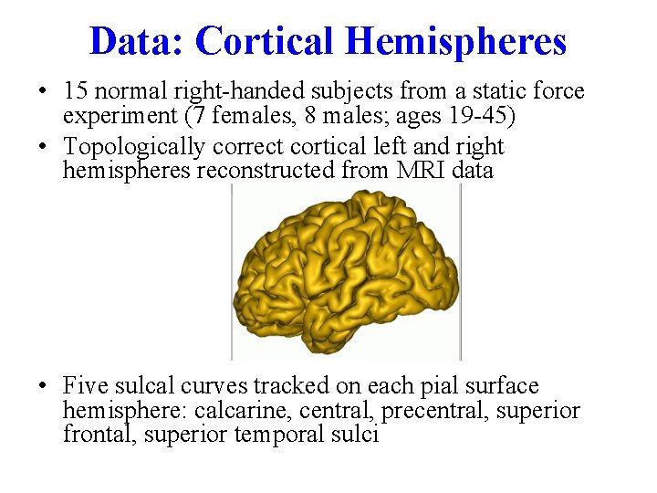
Data: Cortical Hemispheres • 15 normal right-handed subjects from a static force experiment (7 females, 8 males; ages 19 -45) • Topologically correct cortical left and right hemispheres reconstructed from MRI data • Five sulcal curves tracked on each pial surface hemisphere: calcarine, central, precentral, superior frontal, superior temporal sulci

Methodology Superior Frontal sulcus (0. 3, 0. 5, … … … 0. 7) Central sulcus Superior Temporal sulcus Brain surface Calcarine sulcus Sulcus paths Vector of Geometric Measures

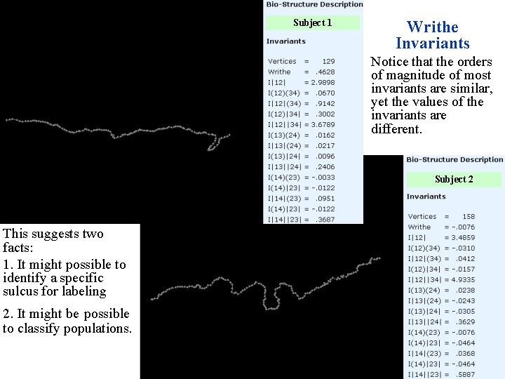
Subject 1 Writhe Invariants Notice that the orders of magnitude of most invariants are similar, yet the values of the invariants are different. Subject 2 This suggests two facts: 1. It might possible to identify a specific sulcus for labeling 2. It might be possible to classify populations.

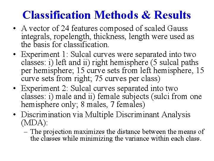
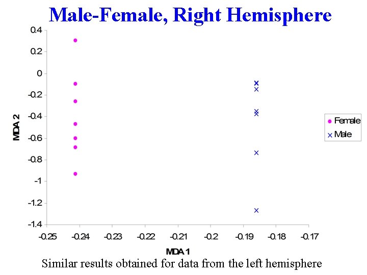
Classification Methods & Results • A vector of 24 features composed of scaled Gauss integrals, ropelength, thickness, length were used as the basis for classification. • Experiment 1: Sulcal curves were separated into two classes: i) left and ii) right hemisphere (5 sulcal paths per hemisphere; 15 curve sets from left hemisphere, 15 curve sets from right; 75 curves per class) • Experiment 2: Sulcal curves separated into two classes: i) male and ii) female subjects (sulci from one hemisphere only; 8 males, 7 females) • Discrimination via Multiple Discriminant Analysis (MDA): – The projection maximizes the distance between the means of the classes while minimizing the variance within each class.

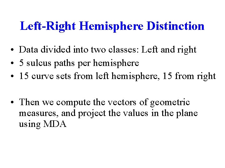
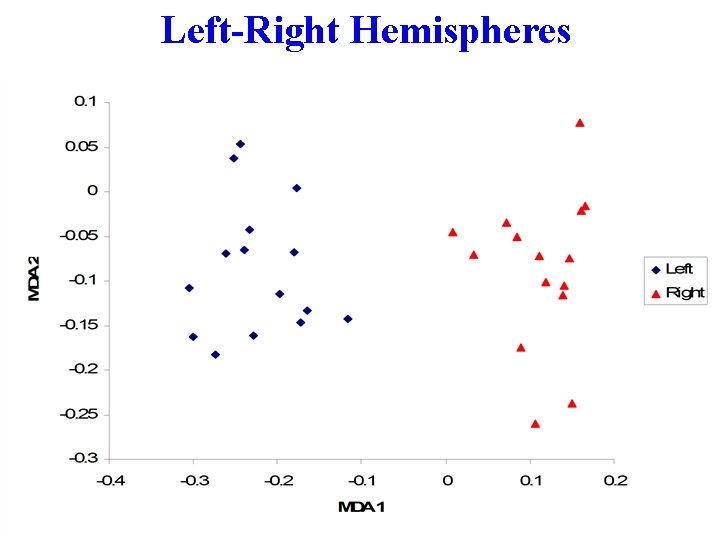
Left-Right Hemisphere Distinction • Data divided into two classes: Left and right • 5 sulcus paths per hemisphere • 15 curve sets from left hemisphere, 15 from right • Then we compute the vectors of geometric measures, and project the values in the plane using MDA

Left-Right Hemispheres

Male-Female Distinction • We divided the data into two classes: Male and Female. • We consider only sulci from one hemisphere (5 sulci per brain). • Compute the vectors of geometric measures, and project by using MDA.

Male-Female, Right Hemisphere Similar results obtained for data from the left hemisphere

Classification Using Machine Learning Methods • MDA results suggest classification scheme possible • WEKA: open source machine learning software • Left-Right Hemisphere: 50% considered for training; a number of methods classified 100% correctly (including Ridor, Lazy LWL) • Male-Female: 75% considered for training; 100% accuracy using Voted Perceptron; 75% accuracy using Ridor; as amount of training decreases, percentage of accuracy drops • Other scenarios, including sulcal curve classification have been successful (see poster)

Conclusions • We used a novel set of geometric measures that seem to capture the anatomy of the brain. • Originally for closed curves, these measures have been extended to open and broken curves. • We perform a number of experiments to test the performance of the Gauss integral measures, length and thickness.

Conclusions • We have a method that could allow a criteria for separating their functional information on the basis of the gross neuroanatomy parameters. • Our method get us one step closer to identify classes of brain anatomy and categorizing function and behavior.

Future Directions • Future direction of this research is to refine the features in order to make discrimination more sensitive, e. g. labeling of sulci on the same hemisphere. • Develop methods that determine which features and algorithms are optimal for classification. These methods need to be tailored to specific applications. • Evaluate robustness of features due to alternate surface reconstructions, other sulci or gyri. • With these invariant features, it might be possible to identify specific sulci for labeling. • Use these measures to differentiate between specific populations.

Acknowledgements Juan Gutierrez, Aaron Kline, Christian Laing, Debbie Smith (Math, FSU) David Rottenberg (Radiology, Neurology, U. Minnesota) for 15 subject MRI data NIH Human Brain Project Grant EB 02013 NSF Focused Research Group Grant DMS-0101329 More information on Brain Mapping: URL: http: //www. math. fsu. edu/~mhurdal Email: mhurdal@math. fsu. edu