Inference for Regression Lines Chapter 12 Conditions LINER

Inference for Regression Lines Chapter 12

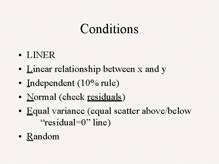
Conditions • • • LINER Linear relationship between x and y Independent (10% rule) Normal (check residuals) Equal variance (equal scatter above/below “residual=0” line) • Random

WE MAY ALWAYS ASSUME ALL CONDITIONS ARE MET (EVEN ON THE AP EXAM)!!!!! WOOT!

Example • Women made significant gains in the 1970’s in terms of their acceptance into professions that had been traditionally populated by men. To measure just how big these gains were, we will compare the percentage of professional degrees award to women in 1972 -1973 to the percentage awarded in 1978 -1979 for selected fields of student from two random samples. (Statistics and Data Analysis, Siegel, Morgan, p. 549)

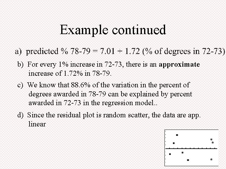
Example continued b) For every 1% increase in 72 -73, there is an approximate increase of 1. 72% in 78 -79. c) We know that 88. 6% of the variation in the percent of degrees awarded in 78 -79 can be explained by percent awarded in 72 -73 in the regression model. . d) Since the residual plot is random scatter, the data are app. linear

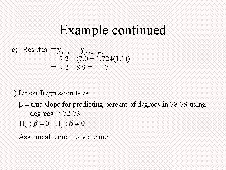
Example continued e) Residual = yactual – ypredicted = 7. 2 – (7. 0 + 1. 724(1. 1)) = 7. 2 – 8. 9 = – 1. 7 f) Linear Regression t-test b = true slope for predicting percent of degrees in 78 -79 using degrees in 72 -73 Assume all conditions are met

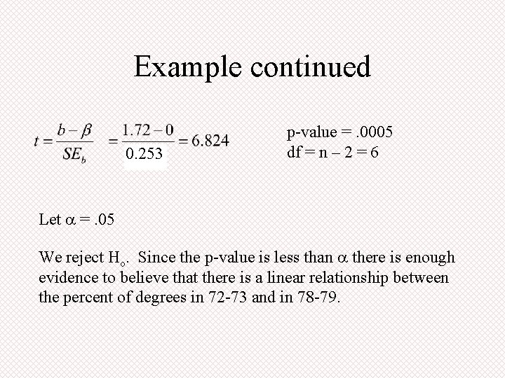
Example continued 0. 253 p-value =. 0005 df = n – 2 = 6 Let a =. 05 We reject Ho. Since the p-value is less than a there is enough evidence to believe that there is a linear relationship between the percent of degrees in 72 -73 and in 78 -79.

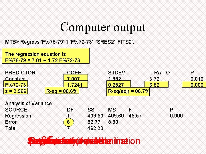
Computer output MTB> Regress ‘F%78 -79’ 1 ‘F%72 -73’ ‘SRES 2’ ‘FITS 2’; The regression equation is F%78 -79 = 7. 01 + 1. 72 F%72 -73 PREDICTOR Constant F%72 -73 s = 2. 966 COEF 7. 007 1. 7241 R-sq = 88. 6% Analysis of Variance SOURCE Regression Error Total DF 1 6 7 STDEV T-RATIO 1. 882 3. 72 0. 2527 6. 82 R-sq(adj) = 86. 7% SS MS F 409. 60 46. 57 52. 77 8. 80 462. 38 SEb of Regression p-value t-score Standard Explanatory Coefficient error of bequation variable determination of the line Estimate a P 0. 010 0. 000 P 0. 000

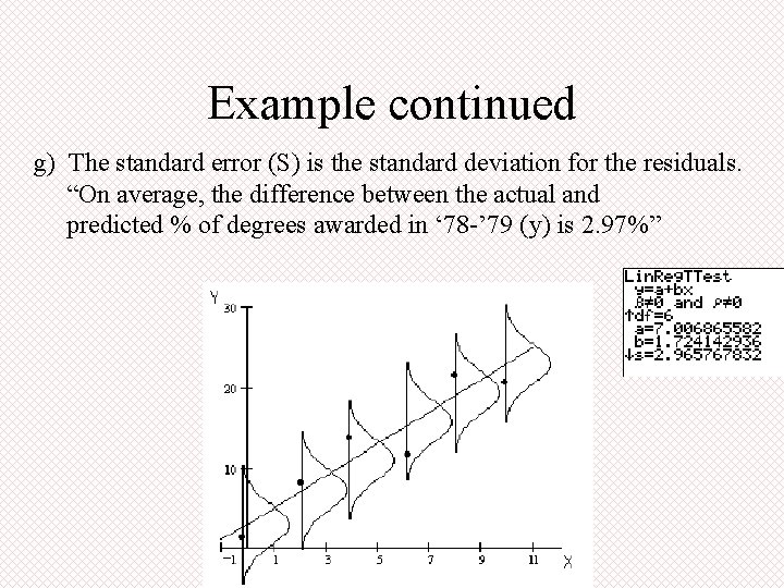
Example continued g) The standard error (S) is the standard deviation for the residuals. “On average, the difference between the actual and predicted % of degrees awarded in ‘ 78 -’ 79 (y) is 2. 97%”

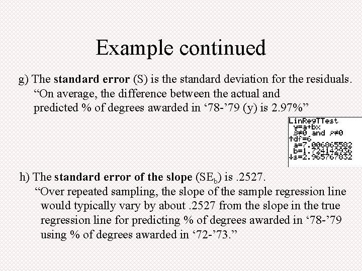
Example continued g) The standard error (S) is the standard deviation for the residuals. “On average, the difference between the actual and predicted % of degrees awarded in ‘ 78 -’ 79 (y) is 2. 97%” h) The standard error of the slope (SEb) is. 2527. “Over repeated sampling, the slope of the sample regression line would typically vary by about. 2527 from the slope in the true regression line for predicting % of degrees awarded in ‘ 78 -’ 79 using % of degrees awarded in ‘ 72 -’ 73. ”

For Your Notes… Standard Error (S) write-up: “On average, the difference between the actual and predicted [y -variable] is [#]. ” Standard Error for the Slope (SEb)write-up: “Over repeated sampling, the slope of the sample regression line would typically vary by about [#] from the slope of the true regression line for predicting [y-variable] using [x-variable]. ”

2) The following is a Mini. Tab output for chocolate shakes using ounces to predict calories. a) On average, the difference between the actual and predicted calories is 50. 80. b) Over repeated sampling, the slope of the sample regression line would typically vary by about 30. 36 from the slope of the true regression line for predicting calories using ounces.

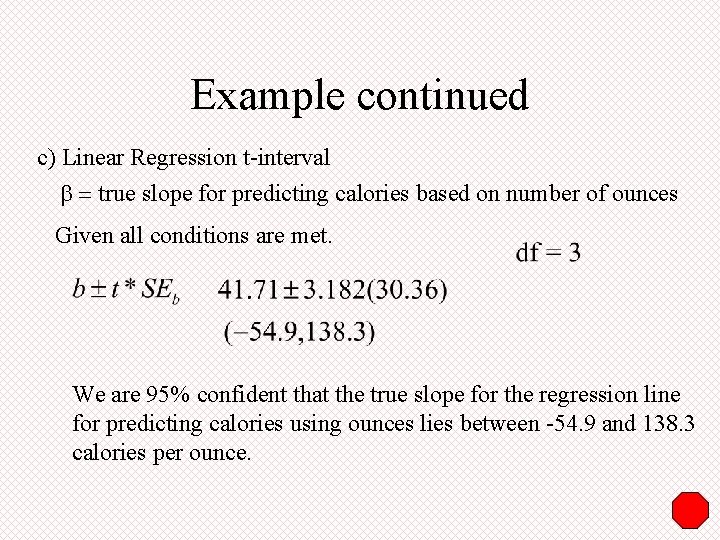
Example continued c) Linear Regression t-interval b = true slope for predicting calories based on number of ounces Given all conditions are met. We are 95% confident that the true slope for the regression line for predicting calories using ounces lies between -54. 9 and 138. 3 calories per ounce.