Inference for regression Simple linear regression IPS chapter

Inference for regression - Simple linear regression IPS chapter 10. 1 © 2006 W. H. Freeman and Company

Objectives (IPS chapter 10. 1) Inference for simple linear regression p Simple linear regression model p Assumptions for inference p Confidence interval for regression parameters p Significance test for the slope p Confidence interval for µy p Inference for prediction

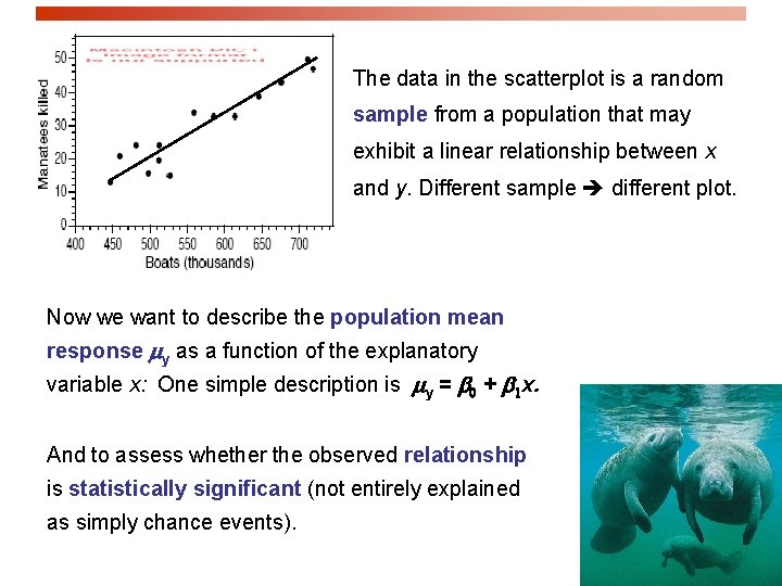
The data in the scatterplot is a random sample from a population that may exhibit a linear relationship between x and y. Different sample different plot. Now we want to describe the population mean response y as a function of the explanatory variable x: One simple description is y = 0 + 1 x. And to assess whether the observed relationship is statistically significant (not entirely explained as simply chance events).

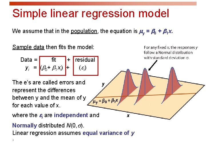
Simple linear regression model We assume that in the population, the equation is y = 0 + 1 x. Sample data then fits the model: Data = fit + residual yi = (b 0+ b 1 xi) + (ei) The e’s are called errors and represent the differences between y and the mean of y for each value of x. where the ei are independent and Normally distributed N(0, ). Linear regression assumes equal variance of y.

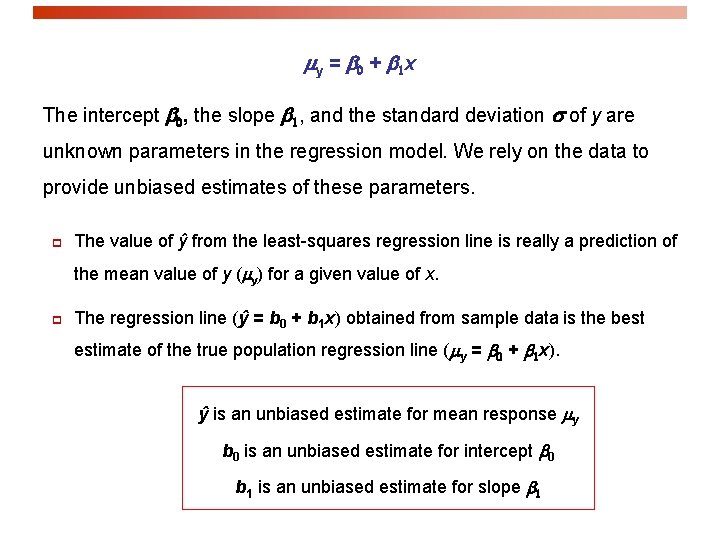
y = 0 + 1 x The intercept 0, the slope 1, and the standard deviation of y are unknown parameters in the regression model. We rely on the data to provide unbiased estimates of these parameters. p The value of ŷ from the least-squares regression line is really a prediction of the mean value of y ( y) for a given value of x. p The regression line (ŷ = b 0 + b 1 x) obtained from sample data is the best estimate of the true population regression line ( y = 0 + 1 x). ŷ is an unbiased estimate for mean response y b 0 is an unbiased estimate for intercept 0 b 1 is an unbiased estimate for slope 1

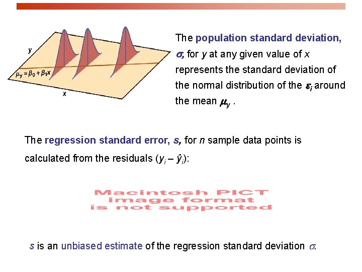
The population standard deviation, for y at any given value of x represents the standard deviation of the normal distribution of the ei around the mean y. The regression standard error, s, for n sample data points is calculated from the residuals (yi – ŷi): s is an unbiased estimate of the regression standard deviation .

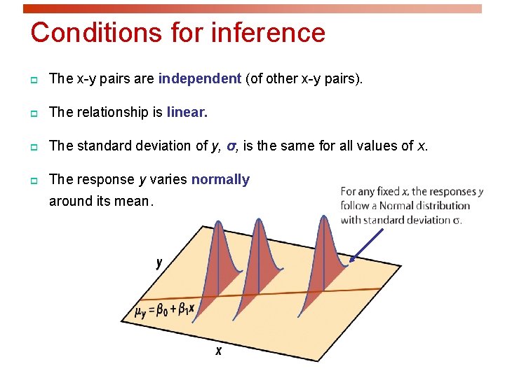
Conditions for inference p The x-y pairs are independent (of other x-y pairs). p The relationship is linear. p The standard deviation of y, σ, is the same for all values of x. p The response y varies normally around its mean.

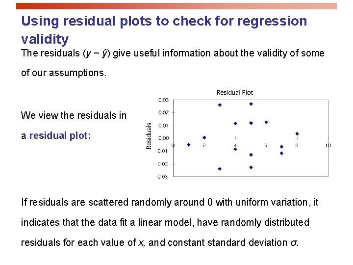
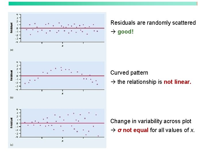
Using residual plots to check for regression validity The residuals (y − ŷ) give useful information about the validity of some of our assumptions. We view the residuals in a residual plot: If residuals are scattered randomly around 0 with uniform variation, it indicates that the data fit a linear model, have randomly distributed residuals for each value of x, and constant standard deviation σ.

Residuals are randomly scattered good! Curved pattern the relationship is not linear. Change in variability across plot σ not equal for all values of x.

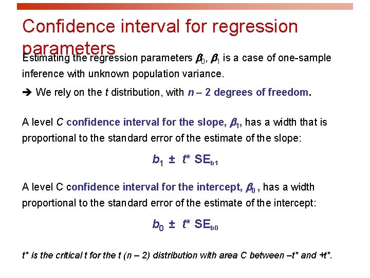
Confidence interval for regression parameters Estimating the regression parameters , is a case of one-sample 0 1 inference with unknown population variance. We rely on the t distribution, with n – 2 degrees of freedom. A level C confidence interval for the slope, 1, has a width that is proportional to the standard error of the estimate of the slope: b 1 ± t* SEb 1 A level C confidence interval for the intercept, 0 , has a width proportional to the standard error of the estimate of the intercept: b 0 ± t* SEb 0 t* is the critical t for the t (n – 2) distribution with area C between –t* and +t*.

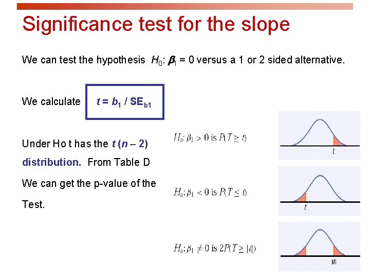
Significance test for the slope We can test the hypothesis H 0: 1 = 0 versus a 1 or 2 sided alternative. We calculate t = b 1 / SEb 1 Under Ho t has the t (n – 2) distribution. From Table D We can get the p-value of the Test.

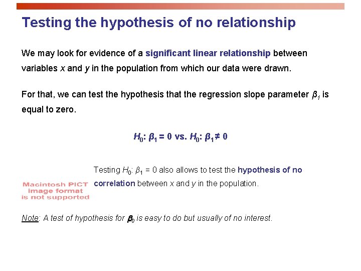
Testing the hypothesis of no relationship We may look for evidence of a significant linear relationship between variables x and y in the population from which our data were drawn. For that, we can test the hypothesis that the regression slope parameter β 1 is equal to zero. H 0: β 1 = 0 vs. H 0: β 1 ≠ 0 Testing H 0: β 1 = 0 also allows to test the hypothesis of no correlation between x and y in the population. Note: A test of hypothesis for 0 is easy to do but usually of no interest.

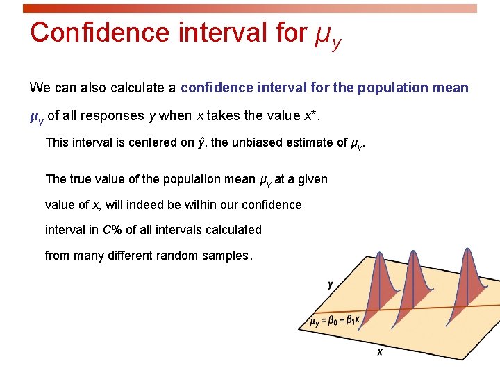
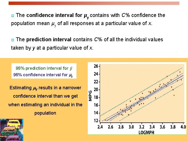
Confidence interval for µy We can also calculate a confidence interval for the population mean μy of all responses y when x takes the value x*. This interval is centered on ŷ, the unbiased estimate of μy. The true value of the population mean μy at a given value of x, will indeed be within our confidence interval in C% of all intervals calculated from many different random samples.

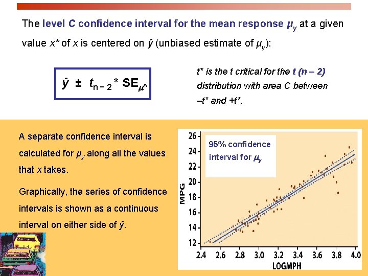
The level C confidence interval for the mean response μy at a given value x* of x is centered on ŷ (unbiased estimate of μy): ŷ ± tn − 2 * SE ^ t* is the t critical for the t (n – 2) distribution with area C between –t* and +t*. A separate confidence interval is calculated for μy along all the values that x takes. Graphically, the series of confidence intervals is shown as a continuous interval on either side of ŷ. 95% confidence interval for y

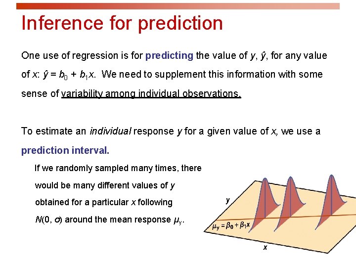
Inference for prediction One use of regression is for predicting the value of y, ŷ, for any value of x: ŷ = b 0 + b 1 x. We need to supplement this information with some sense of variability among individual observations. To estimate an individual response y for a given value of x, we use a prediction interval. If we randomly sampled many times, there would be many different values of y obtained for a particular x following N(0, σ) around the mean response µy.

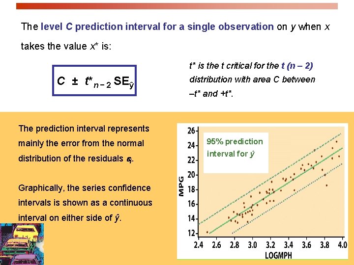
The level C prediction interval for a single observation on y when x takes the value x* is: t* is the t critical for the t (n – 2) C ± t*n − 2 SEŷ distribution with area C between –t* and +t*. The prediction interval represents mainly the error from the normal 95% prediction distribution of the residuals ei. interval for ŷ Graphically, the series confidence intervals is shown as a continuous interval on either side of ŷ.

p The confidence interval for μy contains with C% confidence the population mean μy of all responses at a particular value of x. p The prediction interval contains C% of all the individual values taken by y at a particular value of x. 95% prediction interval for ŷ 95% confidence interval for y Estimating y results in a narrower confidence interval than we get when estimating an individual in the population