HRP 223 2007 lm ppt Linear Models Copyright

HRP 223 – 2007 lm. ppt Linear Models Copyright © 1999 -2007 Leland Stanford Junior University. All rights reserved. Warning: This presentation is protected by copyright law and international treaties. Unauthorized reproduction of this presentation, or any portion of it, may result in severe civil and criminal penalties and will be prosecuted to maximum extent possible under the law.

ANOVA as a Model HPR 223 2007 lm. ppt z At this point, you have seen how you can build a model to describe the mean level of an outcome variable if the predictor is categorical. y You predict the outcome at a baseline level and then add something (a constant) if you are not in the baseline group. After the prediction is made, you are left with some unexplained variability. The extra variability is assumed to be approximately normally distributed with the peak of the bell-shaped curve centered on the mean you guessed.

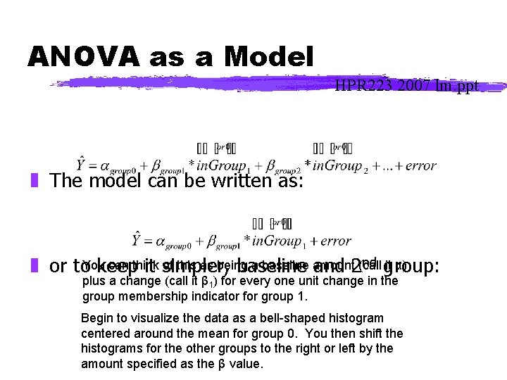
ANOVA as a Model HPR 223 2007 lm. ppt z The model can be written as: nd group: can think of this as being a baseline amount it α) z or to. Youkeep it simpler, baseline and 2(call plus a change (call it β 1) for every one unit change in the group membership indicator for group 1. Begin to visualize the data as a bell-shaped histogram centered around the mean for group 0. You then shift the histograms for the other groups to the right or left by the amount specified as the β value.

From the Last Slide HPR 223 2007 lm. ppt “You can think of this as being a baseline amount (call it α) plus a change (call it β 1) for every one unit change in the group membership indicator (for group 1). ” z Instead of a binary group membership indicator, put in a predictor variable that can take on any integer value between 0 and 10. What happens? y You shift the bell-shaped curve up (or down if the β is negative).

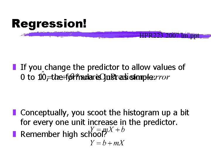
Regression! HPR 223 2007 lm. ppt z If you change the predictor to allow values of 0 to 10, the formula is just as simple. z Conceptually, you scoot the histogram up a bit for every one unit increase in the predictor. z Remember high school?

Continuous Predictors HPR 223 2007 lm. ppt z If you allow your predictor to take on any value and you are comfortable saying you are moving a bell-shaped distribution up or down, you can model the outcome with a line! z Again, the idea is that you are just shifting your best guess at the outcome mean up by some amount (the β) for every one unit increase in the predictor.

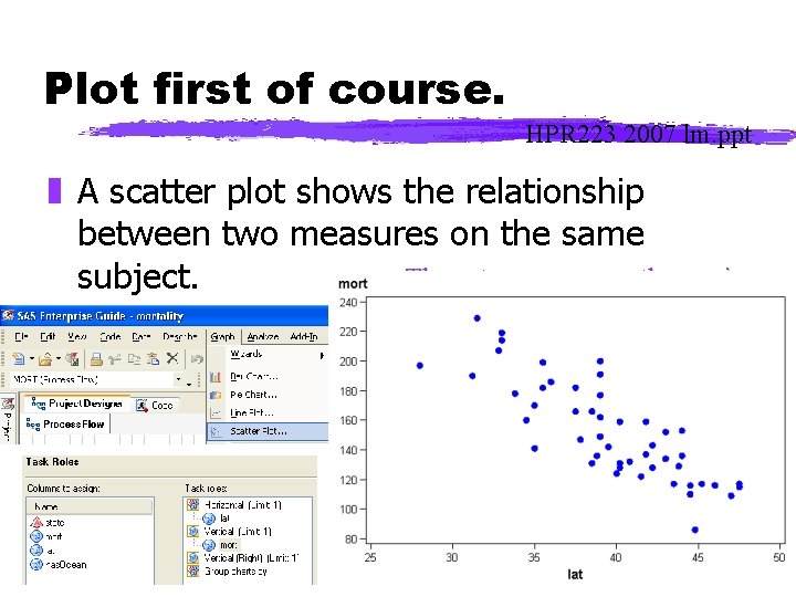
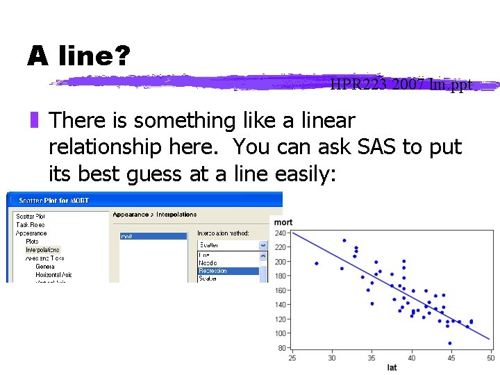
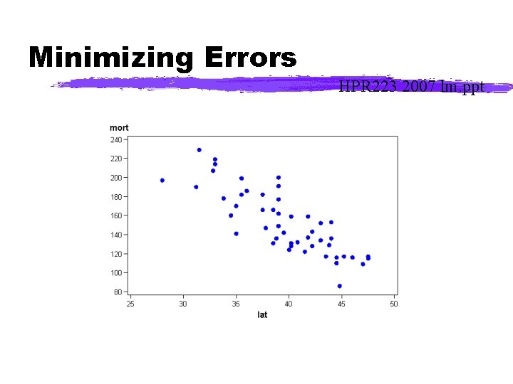
Mortality Rates HPR 223 2007 lm. ppt z Say you want to look at the relationship between mortality caused by malignant melanoma and exposure to sun (as measured by the proxy of latitude). The outcome is mortality. So you will be shifting the distribution of mortality down as latitude goes North.

Plot first of course. HPR 223 2007 lm. ppt z A scatter plot shows the relationship between two measures on the same The outcome goes on the y axis. subject.

A line? HPR 223 2007 lm. ppt z There is something like a linear relationship here. You can ask SAS to put its best guess at a line easily:

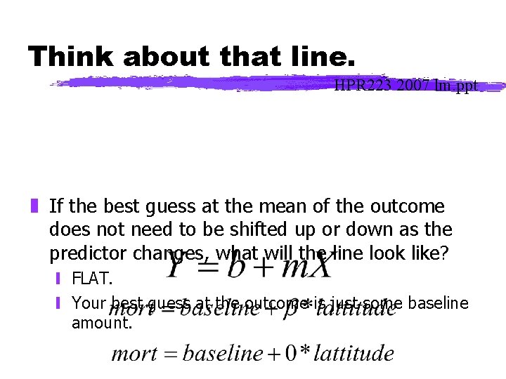
Think about that line. HPR 223 2007 lm. ppt z If the best guess at the mean of the outcome does not need to be shifted up or down as the predictor changes, what will the line look like? y FLAT. y Your best guess at the outcome is just some baseline amount.

Therefore… HPR 223 2007 lm. ppt z The test for the impact of a predictor in a linear model becomes a test of whether the β is close enough to 0 to call it “zero slope”.

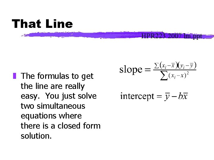
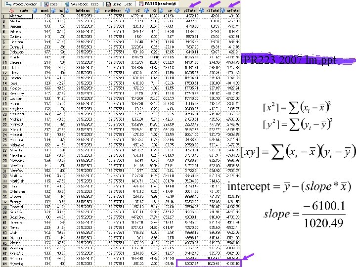
That Line HPR 223 2007 lm. ppt z The formulas to get the line are really easy. You just solve two simultaneous equations where there is a closed form solution.

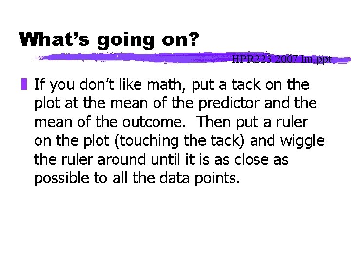
What’s going on? HPR 223 2007 lm. ppt z If you don’t like math, put a tack on the plot at the mean of the predictor and the mean of the outcome. Then put a ruler on the plot (touching the tack) and wiggle the ruler around until it is as close as possible to all the data points.

Minimizing Errors HPR 223 2007 lm. ppt

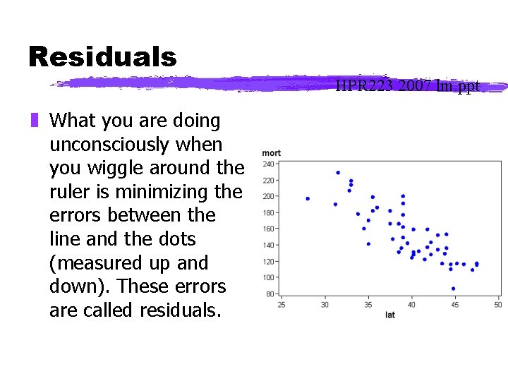
Residuals HPR 223 2007 lm. ppt z What you are doing unconsciously when you wiggle around the ruler is minimizing the errors between the line and the dots (measured up and down). These errors are called residuals.

Guess how you measure error. HPR 223 2007 lm. ppt z Just like every other time you have seen measurements of error, it is expressed as a variance. The model fitting process is just a process of making the line as compatible as possible with the data.

Quality of an ANOVA Model HPR 223 2007 lm. ppt z Remember the ANOVA model is comparing the variance across groups vs. the variance within groups. z Essentially it was saying, do you reduce the variance significantly if you use different mean lines for each subgroup of the data relative to the variance relative to a single mean?

Quality of a Regression Model HPR 223 2007 lm. ppt z Here you are testing to see if the variance is reduced significantly by using a sloped line rather than a flat one.

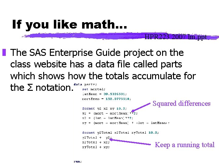
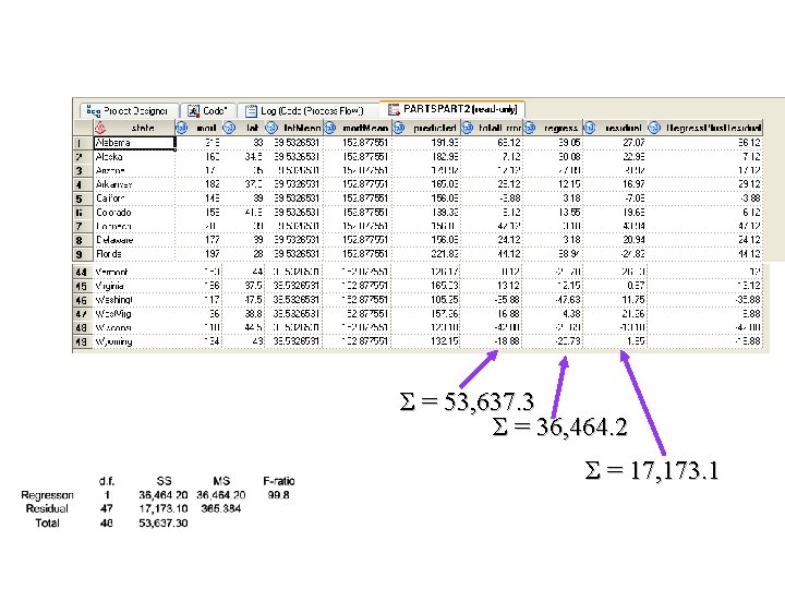
If you like math… HPR 223 2007 lm. ppt z The SAS Enterprise Guide project on the class website has a data file called parts which shows how the totals accumulate for the Σ notation. Squared differences Keep a running total

HPR 223 2007 lm. ppt

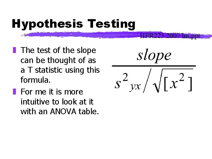
Hypothesis Testing HPR 223 2007 lm. ppt z The test of the slope can be thought of as a T statistic using this formula. z For me it is more intuitive to look at it with an ANOVA table.

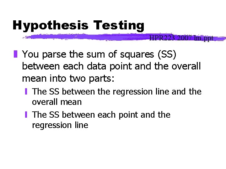
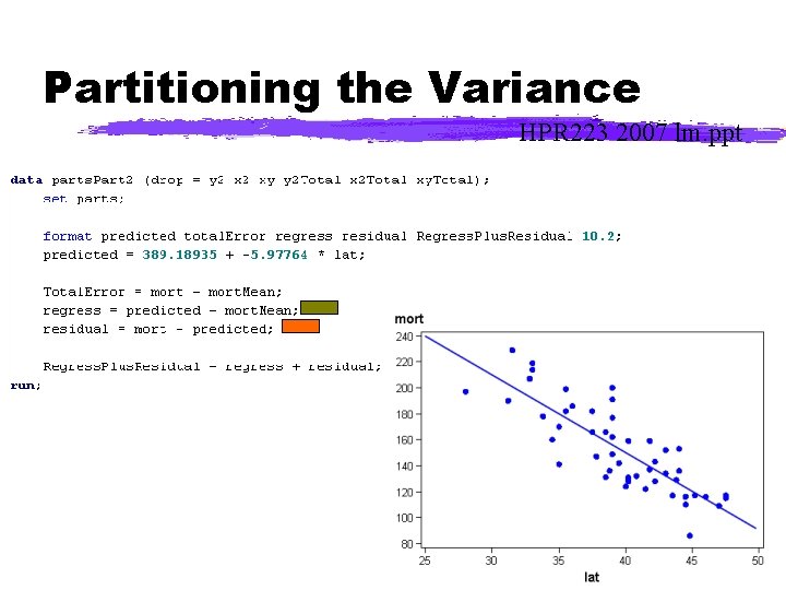
Hypothesis Testing HPR 223 2007 lm. ppt z You parse the sum of squares (SS) between each data point and the overall mean into two parts: y The SS between the regression line and the overall mean y The SS between each point and the regression line

Partitioning the Variance HPR 223 2007 lm. ppt

HPR 223 2007 lm. ppt Σ = 53, 637. 3 Σ = 36, 464. 2 Σ = 17, 173. 1