GROUND MOTION SCALING IN THE MARMARA REGION ATTENUATION

GROUND MOTION SCALING IN THE MARMARA REGION: ATTENUATION OF SEISMIC WAVES (1)M. B. SØRENSEN, (2) A. 1. 2. 3. (3)R. AKINCI, (2) L. MALAGNINI and B. HERRMANN (1) Department of Earth Science, University of Bergen, 4. 5. Allegaten 41, 5007 Bergen, Norway (2) Istituto Nazionale di Geofisica e Vulcanologia 6. Via di Vigna Murata 605, 00143 Roma-Italy (3) Earth and Atm. Sci. Dept. , Saint Louis University, 3507 Laclede Ave. St. Louis MO, USA 7.

WHY THIS STUDY. . . ? § In Seismic Hazard calculations, attenuation is an important input; § Since regional variations in the high-frequency crustal attenuation may be significant, studies on the groundmotion scaling at a regional scale must be performed in order to produce reliable hazard maps;

Tectonic Map of Turkey

A fundamental requirement for hazard studies n is the determination of the ground motion predictive relationships (Kramer, 1996). n Attenuation relationships have been developed for many regions of the world (Ambraseys, 1996; Boore and Joyner, 1991; Boore, 1983; Toro and Mc. Guire, 1987; Atkinson and Boore, 1995; Atkinson and Silva, 1987; Campell, 1997; Sadigh, 1997) mainly by regressing strong- motion data.

Problem: § Strong-motion waveforms are usually not available in large numbers: can we use data from the background seismicity? Solution: § Yes, in this study, we deal mostly with ground velocity data from a set of local recordings. . !

For the evaluation of the seismic hazard we need a predictive relationship for the ground motion: l. Source spectrum l. Crustal attenuation l. Surface geology and topography A general form for a predictive relationship may be: log A(M, r, f)=SOURCE(M, f) + D(r, f) + SITE(f) D(r, f) contains both the geometrical spreading and the anelastic attenuation experienced by the seismic waves all along their paths.

Amplitude A(M, r, f) can be: n n Time-domain quantities (peak ground accelerations, peak ground velocities, response spectra); Frequency-domain quantities (Fourier spectra); in this study, linear predictive relationships are obtained through regressions on data set of ground motion time histories

Time-domain processing n n Define a prototype narrow band-pass filter; For each seismogram, at each frequency: n n Apply the filter Take the peak value: PEAK(f)=SRC(f) + D(r, f) + SITE (f) PEAK(f)=log [ Observed Peak ]

Frequency-domain processing At the same set of central frequencies: n on the original seismograms, compute the Fourier amplitude spectrum on a time window of length T, starting at the S-wave onset. Window length varies with central frequency; n for each central frequency, compute the RMS value of the Fourier amplitude within the corners of the corresponding bandpass filter n AMP(f) = SRC(f) + D(r, f) + SITE(f) AMP(f) = log [ rms Fourier amplitude ]

we are able to arrange all our observations (K observations from J earthquakes recorded at I stations) in a large matrix Ok(rij, f) = SRCj(f) + D(rij, f) + SITEi(f) k = 1, 2, . . , K ; j = 1, 2, . . . , J ; i = 1, 2, . . . , I n n Invert for: D(r, f)=Slpl. Dl pl=(r – Rl)/(Rl+1 -Rl) SITEi (f) (Use an L 1 - norm regression SRCj (f) technique) Constraints : Sj SITEi (f) = 0 D(r=rref, f)=0

After the inversion is run at a set of central frequencies, random vibration theory is used to model the empirical estimates of D(r, rref, f) and SRC(r, rref) RVT combines a random, stationary time history with its Fourier amplitude spectrum and duration to predict its peak value in the time domain. Theory is taken from Cartwright and Longuet. Higgins (1956);

The regional propagation term (normalized) n n n 10 D(ri, rref f)=[g (rij) / g (rref)] exp[-p f (rij – rref) / Q(f)b] g(r) = Geometrical spreading function Q(f) = Qo(f/fref) n Crustal quality factor b= Shear – wave velocity rref= Arbitrary reference distance Let data define crustal attenuation: for the inversion, D(r, rref, f) is parameterised as a piece-wise linear function with many nodes: no a priori assumptions

The last step in the processing is the modelling of the inverted excitation terms Horizontal Velocity Spectrum at reference distance 10 EXCj(rref, f)=sj(f) g(rref) exp(-pfrref /Q(f)b ) <v(f)exp(-pkof)>avg exc(f, rref)= C(2 pf)Mos(f)n(f)p(rref, f) exp(-pkof) s(f) = (1 - e) / (1 + (f/fa)2) + e / (1 + (f/fb)2) C = (0. 55) (0. 707)(2. 0)/4 prb 3 n(f) = generic site amplification factor relative to hard rock p (r, f) = [ g(r) exp ( -pfr/b. Q(f) ) ]

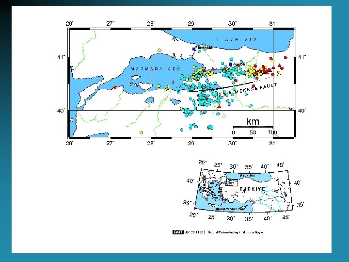
MARMARA REGION 264 Horizontal waveforms (1 station) 100 horizontal waveforms (2 stations) 80 horizontal waveforms (15 stations) Distribution is bad……!

Distance range and magnitudes should be well distributed. . .

Duration of the ground motion as a function of central frequency and hypocentral distance, used as input in RVT

Regional crustal attenuation of ground motion due to geometrical spreading and Q(f) • Horizontal lines represent a 1/r decay with hypocentral distance. • Peak values are modeled through the use of Random Vibration Theory (RVT), given an arbitrary spectral model and an empirical functional form to quantify the duration of ground shaking at each hypocentral distance. • g(r) is forced to be ~ 1/r at short distances and ~ 1/sqrt(r) at large distances. At intermediate r’s, crustal bounces may interfere with direct arrivals, giving rise to complex attenuation patterns. D(r, rref, f)=log g(r) – log(rref) – [pf(r – rref)/b. Q(f)]log e

Modelling the ground motion: geometrical spreading and Q(f) D(r, rref, f)=log g(r) – log(rref) – [pf(r – rref)/b. Q(f)]log e g(r)= r-1. 0, r-0. 6, r-1. 0, r-2. 0, r< 30 km Trade-off: 30 < r < 40 km Since the range of distances is finite, a tradeoff exists 40 < r < 50 km between Q 0 and g(r). r-0. 7, 50 < r < 70 km How to minimize it: r> 70 km…? Force geometrical Q(f)= 300(f/1. 0)0. 3…………. . ? spreading to describe bodywaves at short distances, and surface-waves beyond a critical distance.

Vertical excitation terms at 40 km hypocentral distance Single corner-frequency Brune’s spectral model: Ds=20 Mpa…. . ? k 0=0. 06 sec……? n(f)=1. 0

Vertical site terms are forced to be zero -average at each single frequency: as a consequence of this constraint, possible systematic effects acting on every station are automatically forced over the empirical, vertical excitation terms.

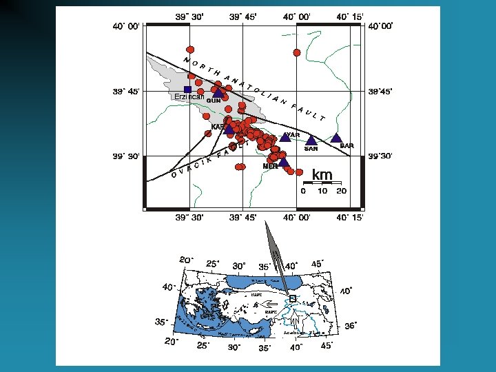
TURKEY (ERZINCAN) 170 recorded earthquakes 743 horizontal waveforms 6 three-component stations

D(r, rref, f)=log g(r) – log(rref) – [pf(r – rref)/b. Q(f)]log e Q(f) = 45 (f/1. 0) 0. 45 g (r) = r – 1. 1 r < 25 km r-0. 5 r > 25 km

k=0. 02 sec Ds=100 bar n(f)=1. 0

SUMMARY k (sec) Ds (bar) Region Q 0 n rmax Colfiorito-Italy 130 0. 10 0. 04 200 50 Apennines-Italy 130 0. 10 0. 00 200 400 Friuli-Italy 300 0. 43 0. 03 600 200 Central Europe 400 0. 42 0. 08 -. 05 30 600 Greece 180 0. 30 0. 06 56 500 Crete 280 0. 25 0. 04 100 200 S. California 180 0. 45 0. 04 70 500 Erzincan –Turkey 45 0. 02 100 40

How do we use these results? n n n We can calibrate linear predictive relationships (LPR) for the ground motion on the regions of interest (examples are next. . . ); We can integrate them into procedures of hazard analysis (coming up!); We make engineers a little happier, by significantly reducing uncertainties in our predictions;

Peak Horizontal Ground Acceleration (g) Squares KOCAELI ERTHQUAKE, 1999, M=7. 4 Other CURVES M=7. 0 PHA’s and PHV’s were computed in each specific region through the use of Random Vibration Theory (RVT), given the attenuation characteristics of the crust, the specific source spectral model, and a functional form which predicts duration of the ground shaking at each epicentral distance (and frequency)

CONCLUSIONS n n n Regionalization shows substantial variations in the attenuation parameters, even within a relatively small country like Italy; Variations must be taken into account in order to produce reliable hazard maps; Regional ground motion scaling can be properly defined by using the background seismicity;

Ds and k trade off Since small events are insensitive to Ds in the frequency band of our interest, they can be used to calibrate k 0. Spectra of radiated energy of large earthquakes, on the other hand, must be used to calibrate the stress parameter. Of course, Ds is expected to change as a function of magnitude.

In the L-1 norm, we no longer need the distributions of residuals to be symmetrically distributed around zero. Since a large number of residuals always characterize the data sets, the medians of the distributions are always very stable quantities, even in cases like the ones shown below. Peak amplitudes: residuals at all central frequencies (fc=0. 25 – 14. 0 Hz)