Genetic Algorithms with Multiple Crossovers on Traveling Salesman

Genetic Algorithms with Multiple Crossovers on Traveling Salesman Problem Paulo Lafeta Ferreira Introduction to Artificial Intelligence – CS 581 Professor: Pushpak Karnick

Introduction to Traveling Salesman Problem (TSP) “Traveling Salesman” must visit each city exactly once and then return back to the starting point. Complexity of the problem (NP-hard) grows exponentially. Approximate solutions can be made using Genetic Algorithms.

Djibouti Map: 89 cities: http: //www. tsp. gatech. edu

Djibouti Optimal solution found. Path size: 351 mi

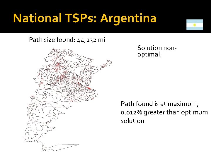
National TSPs: Argentina Map: 9, 152 Cities:

National TSPs: Argentina Path size found: 44, 232 mi Solution nonoptimal. Path found is at maximum, 0. 012% greater than optimum solution.

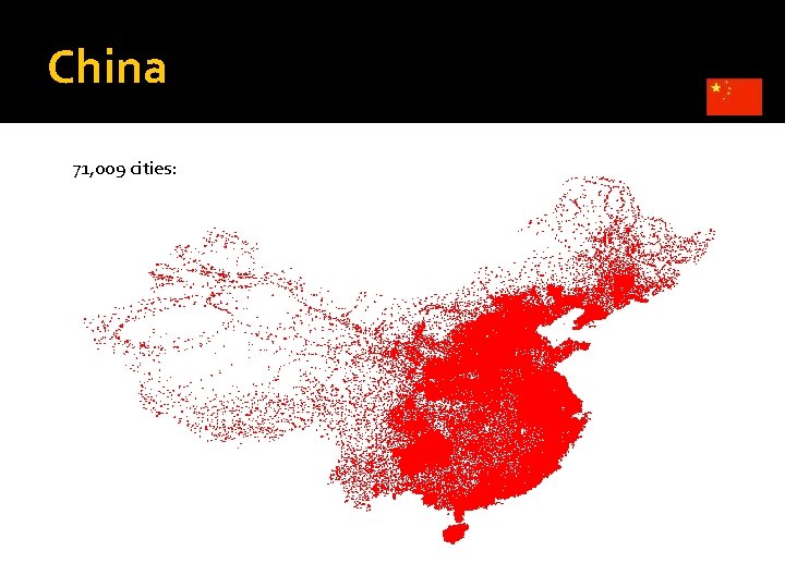
China Map:

China 71, 009 cities:

China Best path found in a recent test:

China Path size: 241, 188 mi 0. 024% near optimal solution

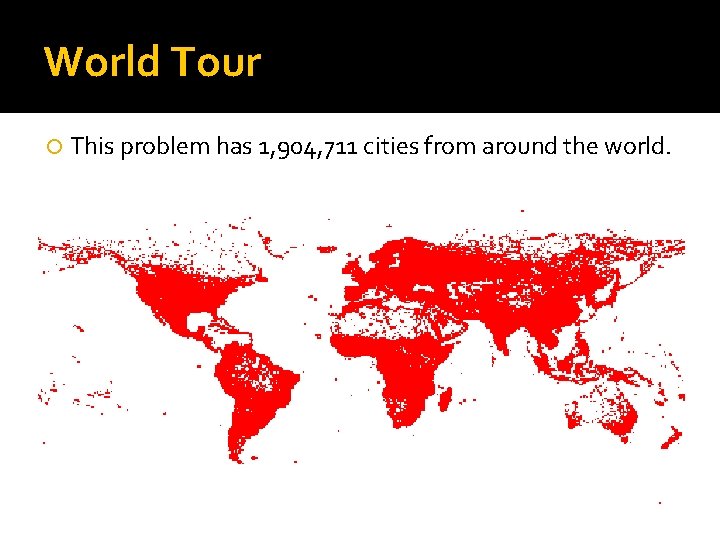
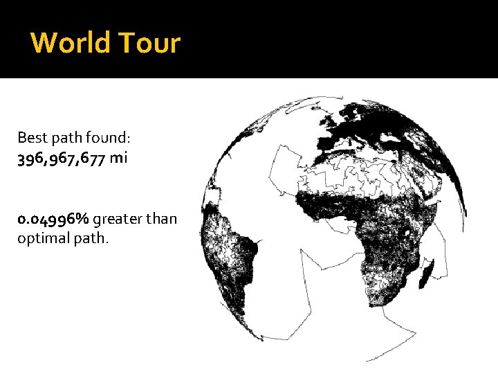
World Tour This problem has 1, 904, 711 cities from around the world.

World Tour Best path found: 396, 967, 677 mi 0. 04996% greater than optimal path.

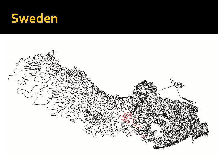
Bigger National TSP solved Sweden: 24, 978 cities Path size: 45, 049 mi Used 96 clusters dual Intel Xeon 2. 8 Ghz Time running: approximately 3 years In an usual computer: ~84 years

Sweden

Crossovers implemented Path Crossovers: ▪ Partially Mapped (PMX) ▪ Order (OX) ▪ Cycle (CX) Ordinal Crossover: ▪ Cut-and-splice Adjacency Crossovers: ▪ Alternating Edges ▪ Subtour-chunks ▪ Heuristic

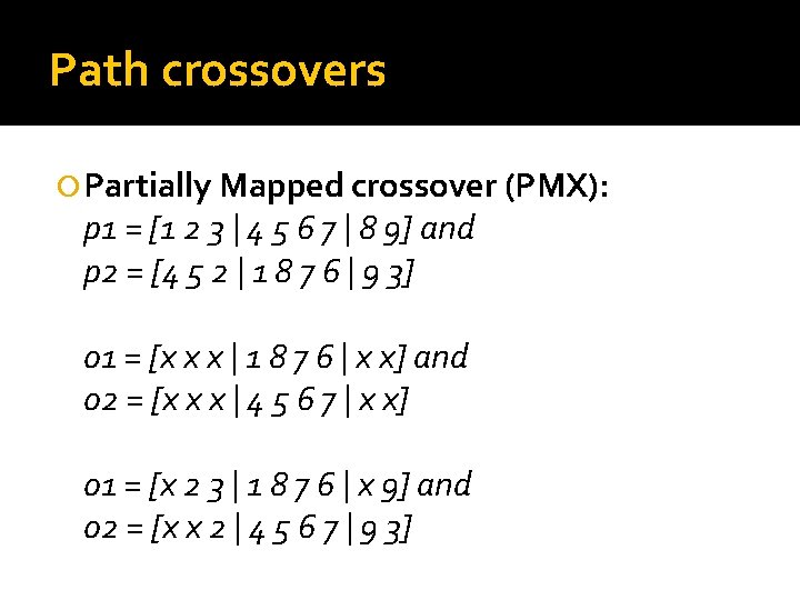
Path crossovers Partially Mapped crossover (PMX): p 1 = [1 2 3 | 4 5 6 7 | 8 9] and p 2 = [4 5 2 | 1 8 7 6 | 9 3] o 1 = [x x x | 1 8 7 6 | x x] and o 2 = [x x x | 4 5 6 7 | x x] o 1 = [x 2 3 | 1 8 7 6 | x 9] and o 2 = [x x 2 | 4 5 6 7 | 9 3]

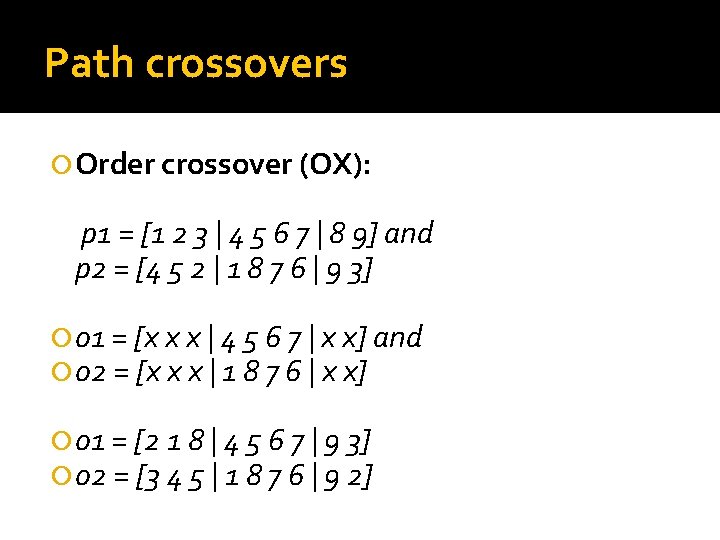
Path crossovers Order crossover (OX): p 1 = [1 2 3 | 4 5 6 7 | 8 9] and p 2 = [4 5 2 | 1 8 7 6 | 9 3] o 1 = [x x x | 4 5 6 7 | x x] and o 2 = [x x x | 1 8 7 6 | x x] o 1 = [2 1 8 | 4 5 6 7 | 9 3] o 2 = [3 4 5 | 1 8 7 6 | 9 2]

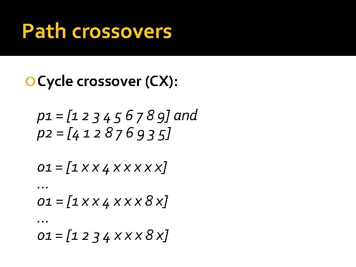
Path crossovers Cycle crossover (CX): p 1 = [1 2 3 4 5 6 7 8 9] and p 2 = [4 1 2 8 7 6 9 3 5] o 1 = [1 x x 4 x x x] … 01 = [1 x x 4 x x x 8 x] … o 1 = [1 2 3 4 x x x 8 x]

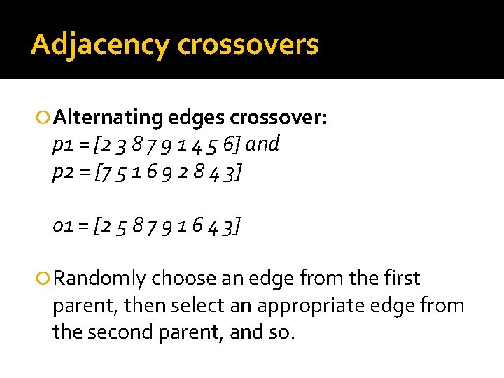
Adjacency crossovers Alternating edges crossover: p 1 = [2 3 8 7 9 1 4 5 6] and p 2 = [7 5 1 6 9 2 8 4 3] o 1 = [2 5 8 7 9 1 6 4 3] Randomly choose an edge from the first parent, then select an appropriate edge from the second parent, and so.

Adjacency crossovers Subtour-chunks crossover Similar to “Alternating Edges”, but instead of switching only one element, switch a random -length subtour from one of the parents.

Adjacency crossovers Heuristic crossover Choose a random city, then compares two edges that emanate from this city from both parents. Choose the one with lower cost. The city on the other end of this edge, is the next starting point.

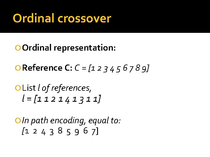
Ordinal crossover Ordinal representation: Reference C: C = [1 2 3 4 5 6 7 8 9] List l of references, l = [1 1 2 1 4 1 3 1 1] In path encoding, equal to: [1 2 4 3 8 5 9 6 7]

Ordinal crossover Cut-and-splice crossover Take a part from one parent, and splice it with the remainder from the second parent.

Strategies used: Elitism Maintain the best individual found so far in the population. Applied only if the population is equal or greater than 4.

Strategies used: Getting out of Local Optima Randomize one or two children when both are equal after reproduction. This increased the performance of the GA in general, due to the high frequency of GA being stuck in a local optima. Other option: randomize entire population if best solution does not change after Y iterations.

Strategies used: Multiple Crossovers After a while, single crossover methods start lacking variety in their reproductions. Possible solutions: Randomize part of the population. and/or: Change crossover method in real time, during execution.

Strategies used: Multiple Crossovers During execution, switch crossover method when “best solution” doesn’t change during n iterations. Conversion of all individuals is necessary if switch is between a Path and an Adjacency crossover. Crossovers used: Heuristic (Adjacency) Partially Mapped (Path) Order (Path) Subtour-chunks (Adjacency)

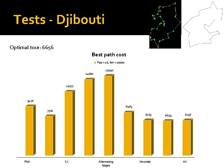
Tests - Djibouti Optimal tour: 6656 Best path cost Pop = 16, Iter = 10000 14620 15290 12277 9470 8285 7561 6765 PMX CX Alternating Edges Heuristic 6659 6758 All

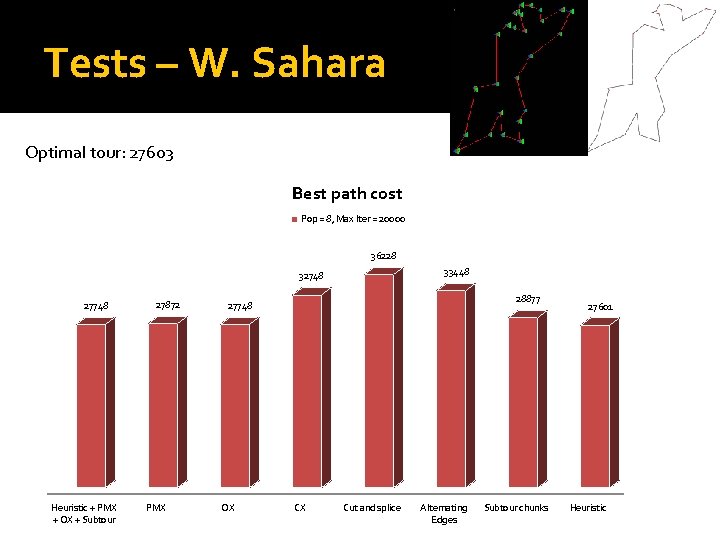
Tests – W. Sahara Optimal tour: 27603 Best path cost Pop = 8, Max Iter = 20000 36228 33448 32748 27748 Heuristic + PMX + OX + Subtour 27872 PMX 28877 27748 OX CX Cut and splice Alternating Edges Subtour chunks 27601 Heuristic

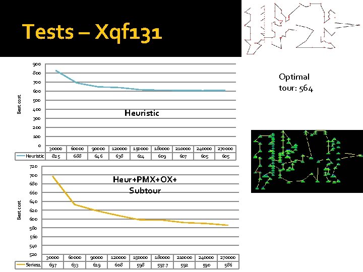
Tests – Xqf 131 Xqf - Heuristic 900 800 Optimal tour: 564 700 Best cost 600 500 400 Heuristic 300 200 100 0 Heuristic 30000 825 60000 688 90000 646 120000 638 150000 614 180000 609 210000 607 240000 605 270000 605 720 700 Heur+PMX+OX+ Subtour 680 Best cost 660 640 620 600 580 560 540 520 Series 1 30000 697 60000 633 90000 619 120000 608 150000 598 180000 597. 7 210000 592 240000 590 270000 586

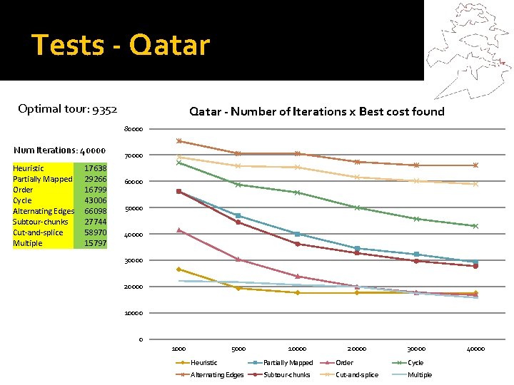
Tests - Qatar Optimal tour: 9352 Qatar - Number of Iterations x Best cost found 80000 Num Iterations: 40000 Heuristic Partially Mapped Order Cycle Alternating Edges Subtour-chunks Cut-and-splice Multiple 17638 29266 16799 43006 66098 27744 58970 15797 70000 60000 50000 40000 30000 20000 10000 0 1000 5000 10000 20000 30000 Heuristic Partially Mapped Order Cycle Alternating Edges Subtour-chunks Cut-and-splice Multiple 40000

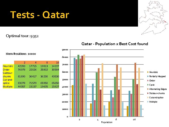
Tests - Qatar Optimal tour: 9352 Qatar - Population x Best Cost found 90000 Num Iterations: 10000 Heuristic Order Subtourchunks Cut-andsplice Multiple 80000 2 42200 76978 4 17715 22026 8 19813 25802 16 14227 30584 81890 36417 36230 43530 83278 44357 71579 15157 65950 19605 65650 15827 70000 60000 Heuristic Partially Mapped 50000 Order Cycle 40000 Alternating Edges Subtour-chunks 30000 Cut-and-splice 20000 Multiple 10000 0 2 4 Population 8 16

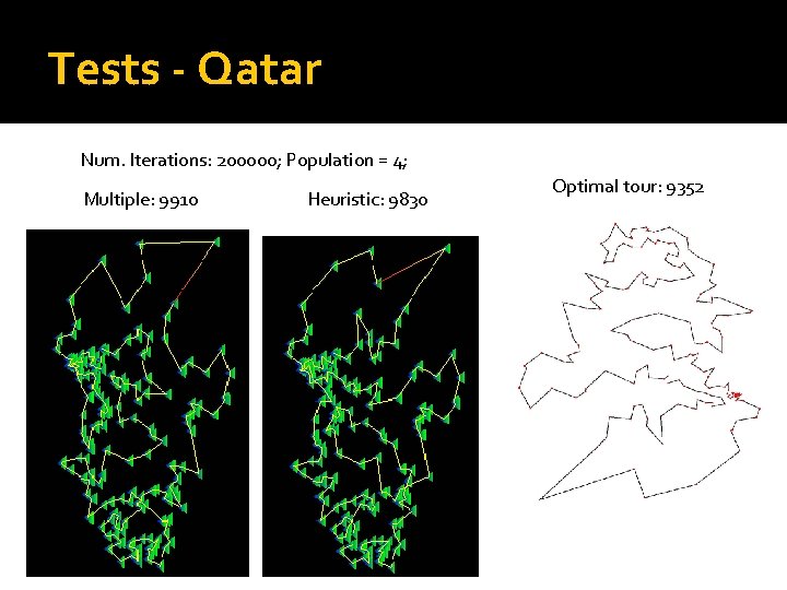
Tests - Qatar Num. Iterations: 200000; Population = 4; Multiple: 9910 Heuristic: 9830 Optimal tour: 9352

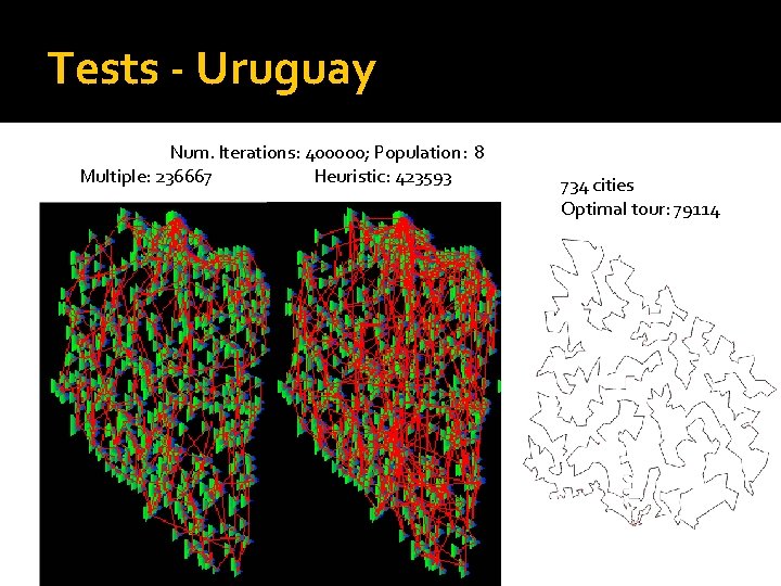
Tests - Uruguay Num. Iterations: 400000; Population: 8 Multiple: 236667 Heuristic: 423593 734 cities Optimal tour: 79114

Conclusion Heuristic showed best performance between the 7 implemented. Converges quickly to a “good” solution But after an amount of iterations it gets “stuck” Followed by the Order. Ordinal with its Cut-and-splice is easy to implement and works well in some GA problems, but not in TSP.

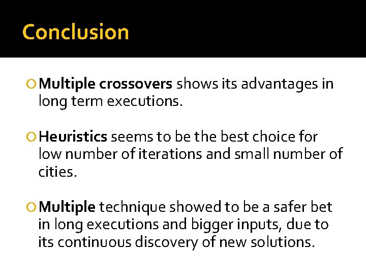
Conclusion Multiple crossovers shows its advantages in long term executions. Heuristics seems to be the best choice for low number of iterations and small number of cities. Multiple technique showed to be a safer bet in long executions and bigger inputs, due to its continuous discovery of new solutions.

Conclusion What might improve the Multiple technique: Store information about crossovers performance during execution and then select the current best techniques more frequently. Vary number of iterations necessary to switch crossover, based on their current performance.

Thank you!