Traveling Salesman Problem TSP Definition Given n points

巡回セールスマン問題って何？ Traveling Salesman Problem (TSP)

Definition Given n points (cities) and a distance function between two points, find a minimum length Hamiltonian circuit a b |ab|=|ba| b a c |ab|=|ba| Symmetric TSP otherwise Asymmetric TSP |ac|≦|ab|+|bc| ΔTSP points are in d-dim. Euclidean space Euclidean TSP

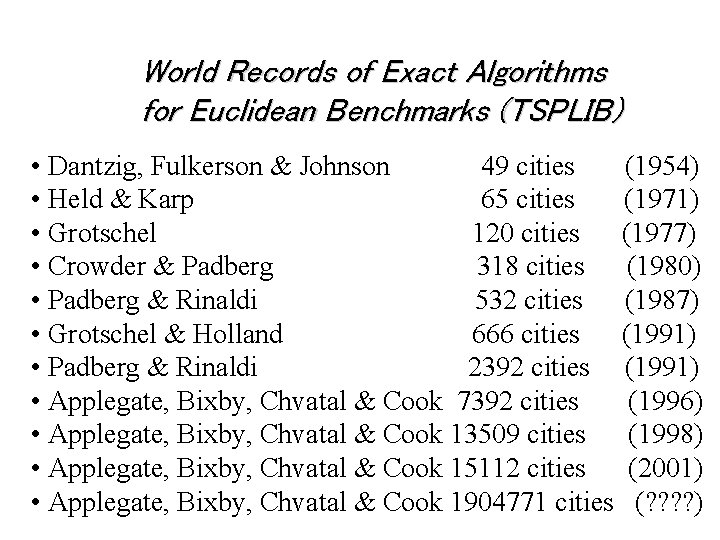
World Records of Exact Algorithms for Euclidean Benchmarks (TSPLIB) • Dantzig, Fulkerson & Johnson 49 cities (1954) • Held & Karp 65 cities (1971) • Grotschel 120 cities (1977) • Crowder & Padberg 318 cities (1980) • Padberg & Rinaldi 532 cities (1987) • Grotschel & Holland 666 cities (1991) • Padberg & Rinaldi 2392 cities (1991) • Applegate, Bixby, Chvatal & Cook 7392 cities (1996) • Applegate, Bixby, Chvatal & Cook 13509 cities (1998) • Applegate, Bixby, Chvatal & Cook 15112 cities (2001) • Applegate, Bixby, Chvatal & Cook 1904771 cities (? ? )

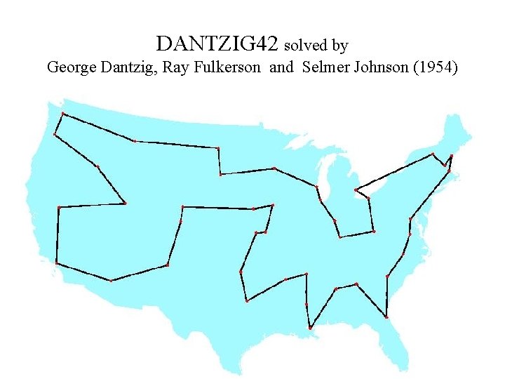
DANTZIG 42 solved by George Dantzig, Ray Fulkerson and Selmer Johnson (1954)

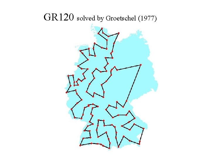
GR 120 solved by Groetschel (1977)

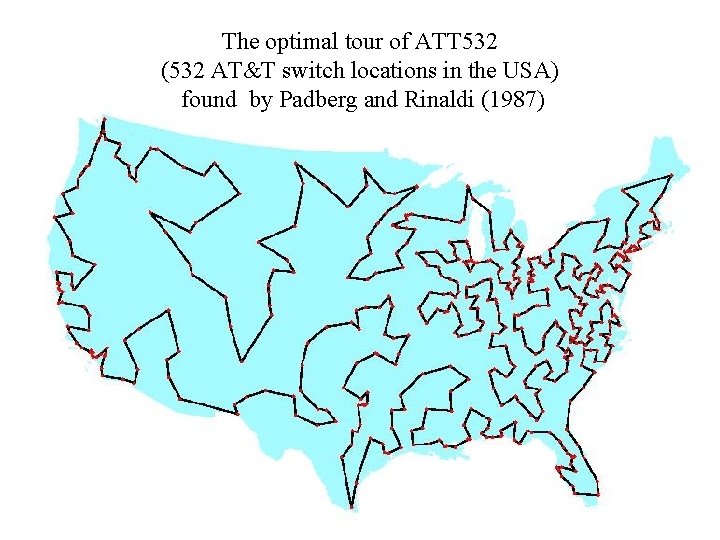
The optimal tour of ATT 532 (532 AT&T switch locations in the USA) found by Padberg and Rinaldi (1987)

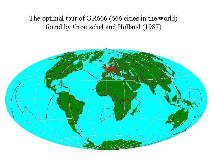
The optimal tour of GR 666 (666 cities in the world) found by Groetschel and Holland (1987)

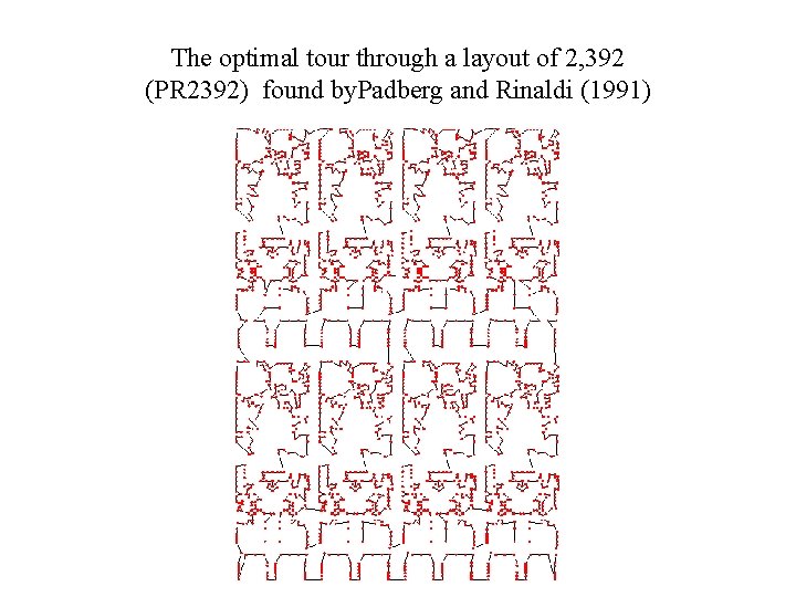
The optimal tour through a layout of 2, 392 (PR 2392) found by. Padberg and Rinaldi (1991)

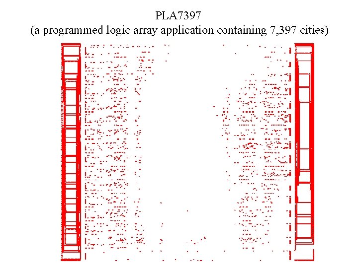
PLA 7397 (a programmed logic array application containing 7, 397 cities)

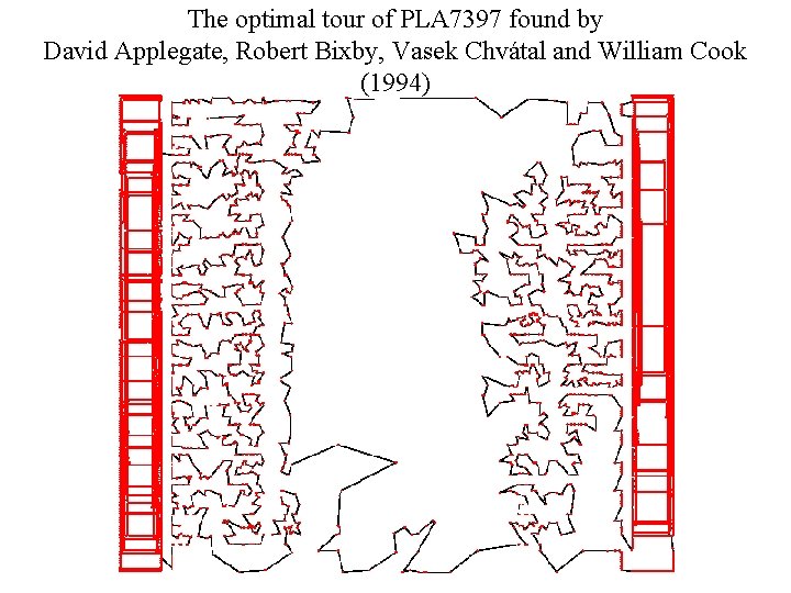
The optimal tour of PLA 7397 found by David Applegate, Robert Bixby, Vasek Chvátal and William Cook (1994)

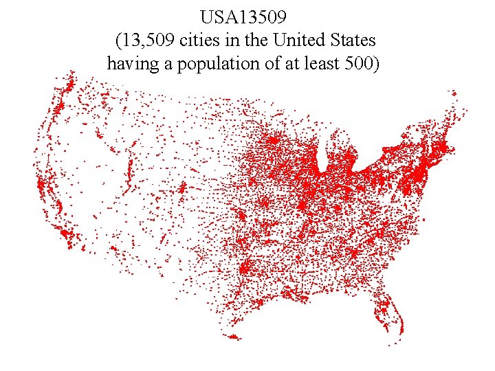
USA 13509 (13, 509 cities in the United States having a population of at least 500)

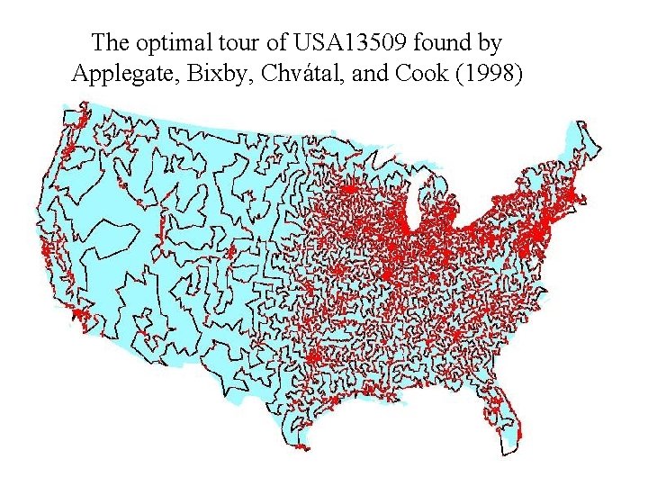
The optimal tour of USA 13509 found by Applegate, Bixby, Chvátal, and Cook (1998)

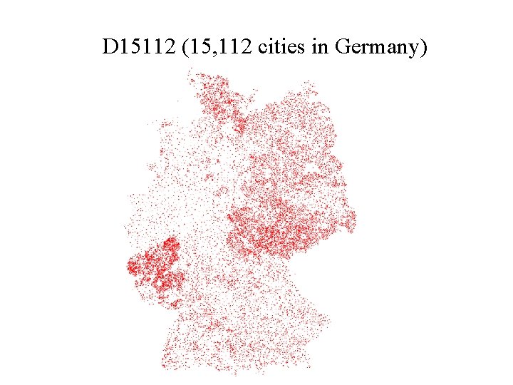
D 15112 (15, 112 cities in Germany)

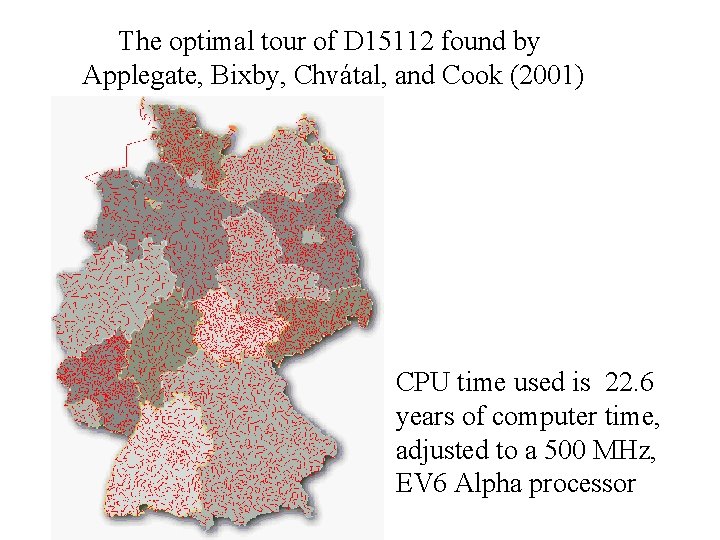
The optimal tour of D 15112 found by Applegate, Bixby, Chvátal, and Cook (2001) CPU time used is 22. 6 years of computer time, adjusted to a 500 MHz, EV 6 Alpha processor

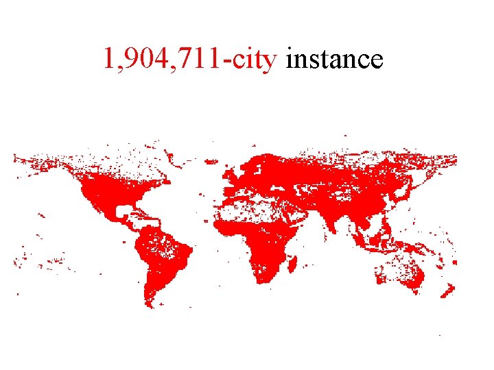
1, 904, 711 -city instance

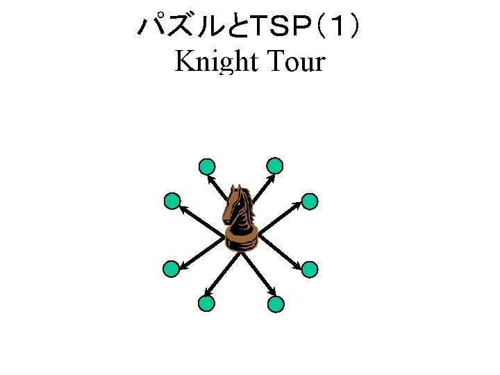
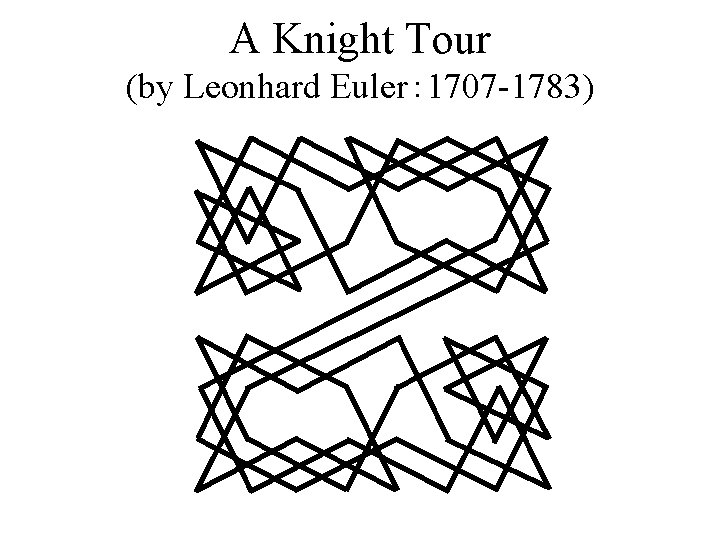
A Knight Tour (by Leonhard Euler： 1707 -1783)

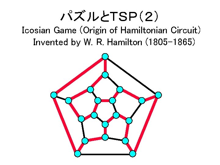
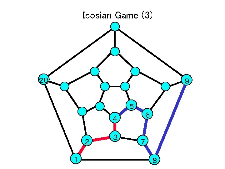
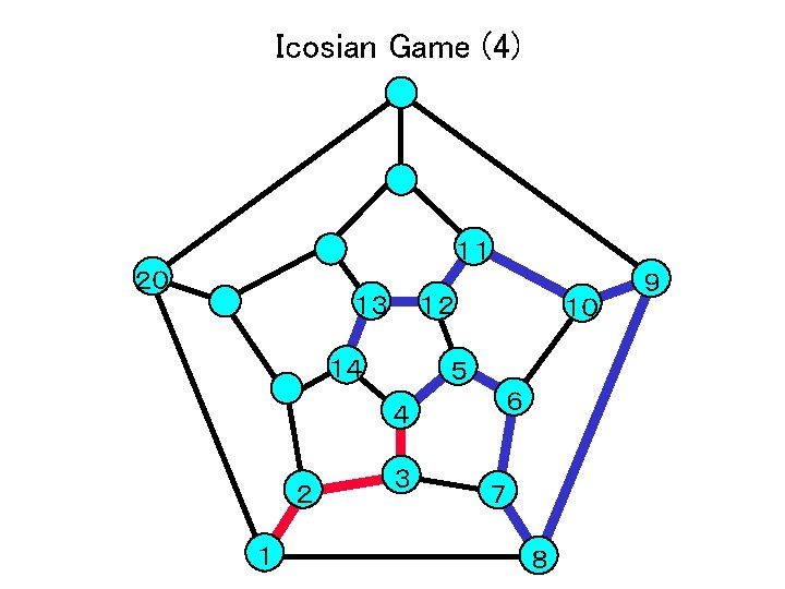
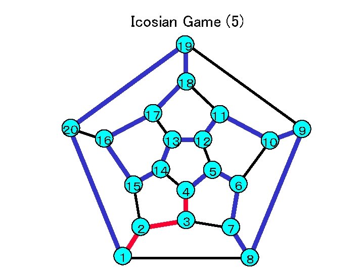
パズルとＴＳＰ（２） Icosian Game (Origin of Hamiltonian Circuit) Invented by W. R. Hamilton (1805 -1865)

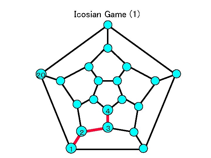
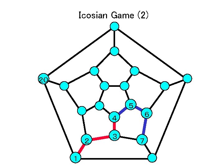
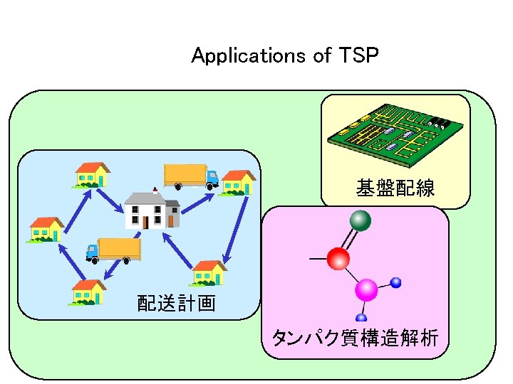
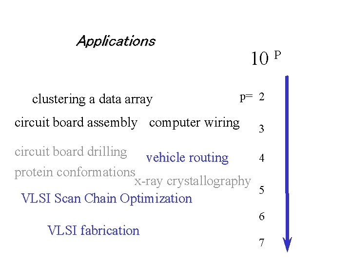
Applications clustering a data array circuit board assembly computer wiring 10 P p= 2 3 circuit board drilling vehicle routing 4 protein conformations x-ray crystallography 5 VLSI Scan Chain Optimization 6 VLSI fabrication 7

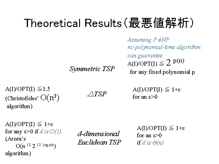
Theoretical Results（最悪値解析） Symmetric TSP A(I)/OPT(I) ≦ 1. 5 (Christofides’ O(n 3) algorithm) A(I)/OPT(I) ≦ 1+ε for any ε>0 if d is O(1) (Arora’s O(n 12 2 13 log n/ε) algorithm) △TSP d-dimensional Euclidean TSP Assuming P ≠NP no polynomial-time algorithm can guarantee A(I)/OPT(I) ≦ p(n) for any fixed polynomial p 2 A(I)/OPT(I) ≦ 1+ε for an ε>0 if d is Θ(n)

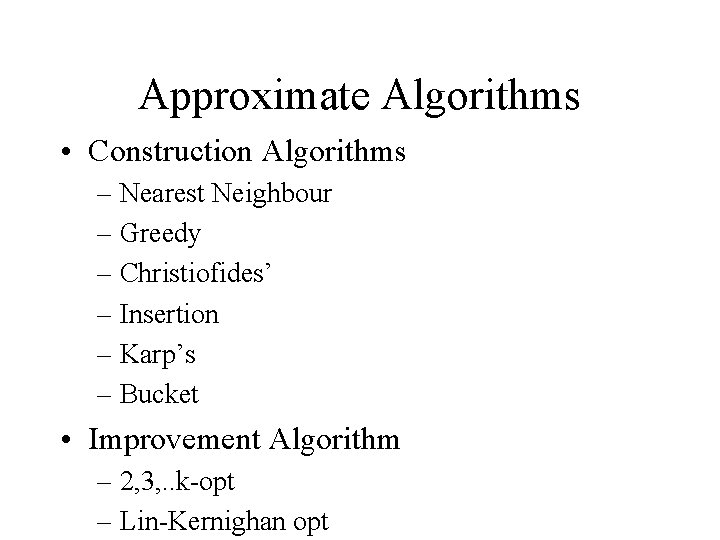
Approximate Algorithms • Construction Algorithms – Nearest Neighbour – Greedy – Christiofides’ – Insertion – Karp’s – Bucket • Improvement Algorithm – 2, 3, . . k-opt – Lin-Kernighan opt

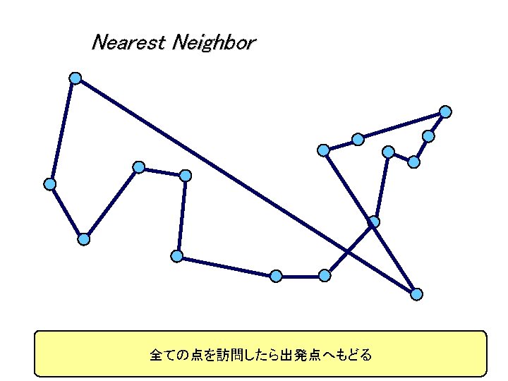
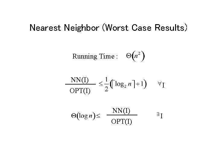
Nearest Neighbor (Worst Case Results) Running Time : NN(I) OPT(I) ∀I NN(I) OPT(I) ∃I

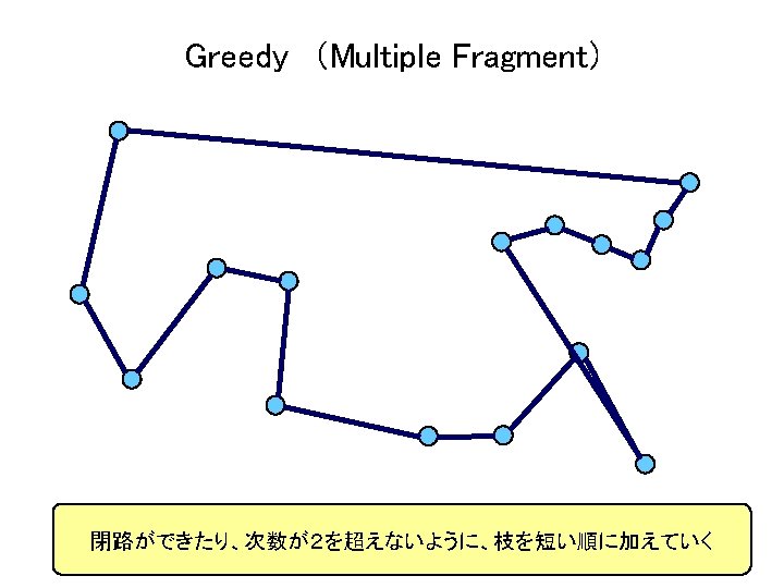
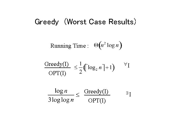
Greedy (Worst Case Results) Running Time : Greedy(I) OPT(I) ∀I Greedy(I) OPT(I) ∃I

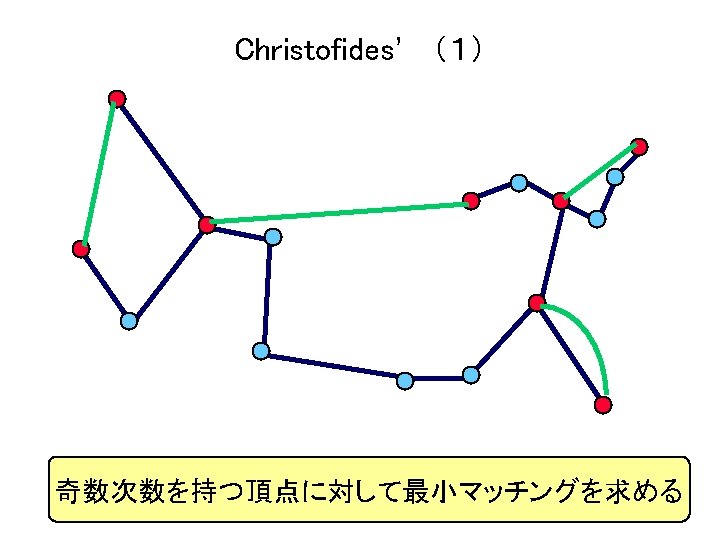
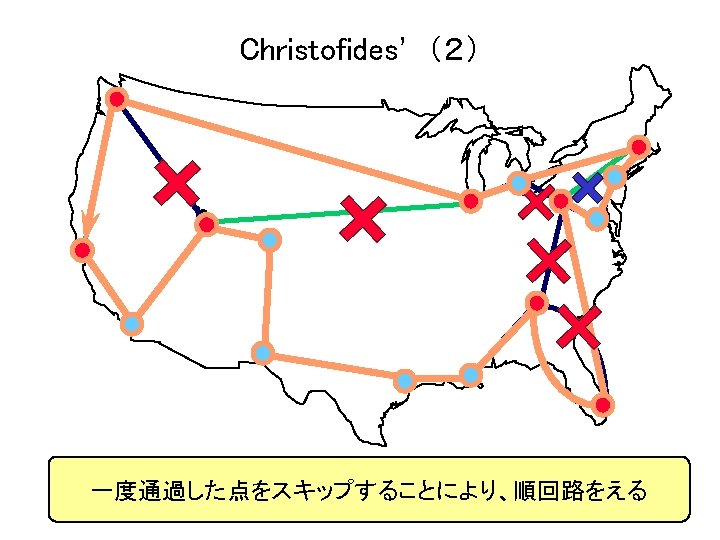
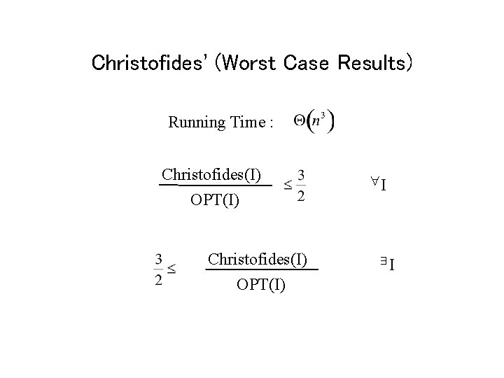
Christofides’ (Worst Case Results) Running Time : Christofides(I) OPT(I) ∀I ∃I

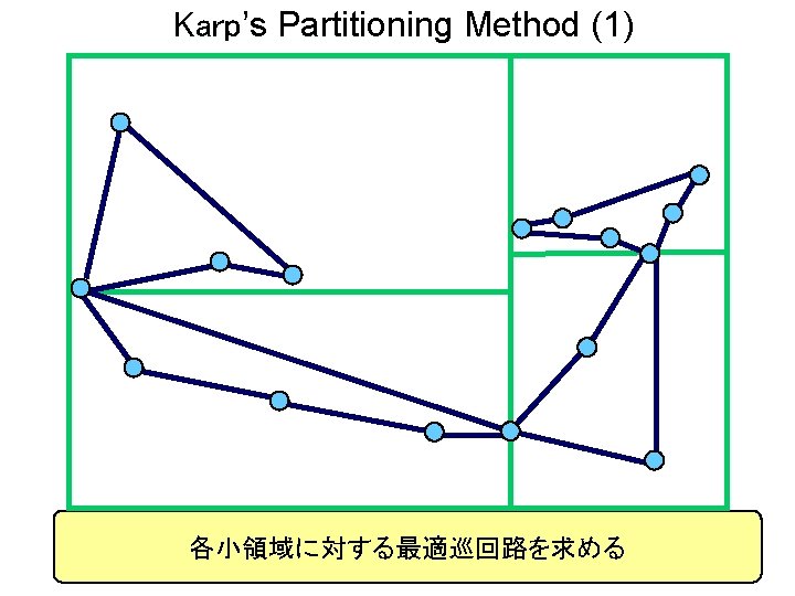
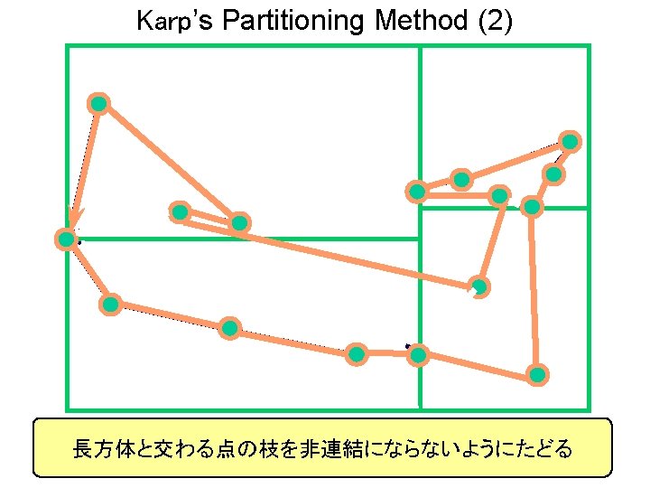
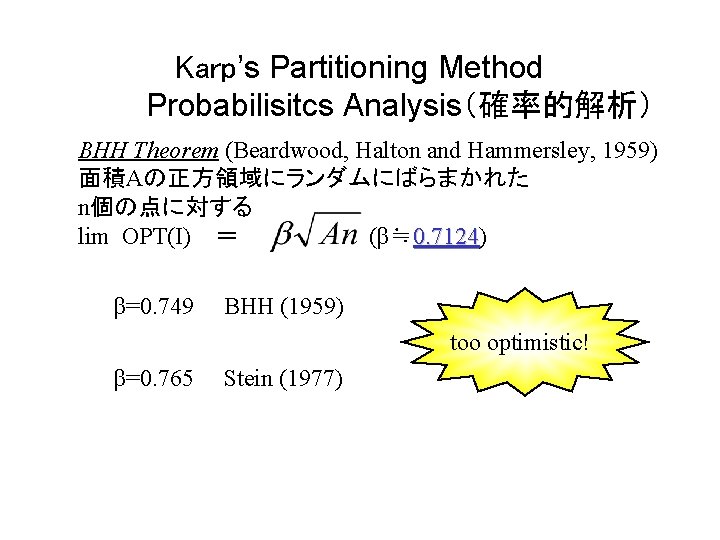
Karp’s Partitioning Method Probabilisitcs Analysis（確率的解析） BHH Theorem (Beardwood, Halton and Hammersley, 1959) 面積Aの正方領域にランダムにばらまかれた n個の点に対する lim OPT(I) ＝ (β≒ 0. 7124) 0. 7124 β=0. 749 BHH (1959) too optimistic! β=0. 765 Stein (1977)

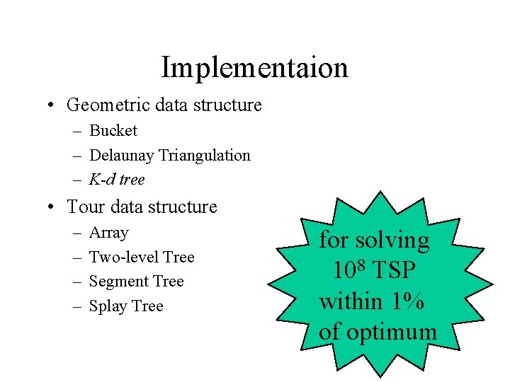
Implementaion • Geometric data structure – Bucket – Delaunay Triangulation – K-d tree • Tour data structure – – Array Two-level Tree Segment Tree Splay Tree for solving 108 TSP within 1% of optimum

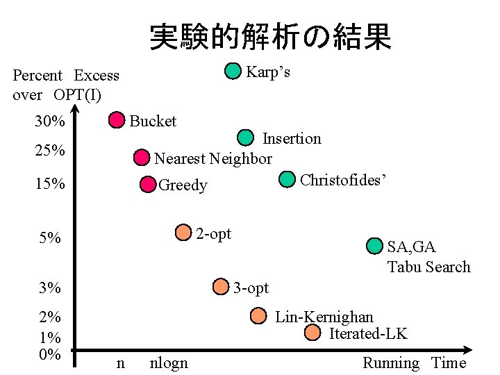
実験的解析の結果 Karp’s Percent Excess over OPT(I) 30% Bucket Insertion Nearest Neighbor Christofides’ Greedy 25% 15% 2 -opt 5% 3% 2% 1% 0% SA, GA Tabu Search 3 -opt Lin-Kernighan Iterated-LK n nlogn Running Time

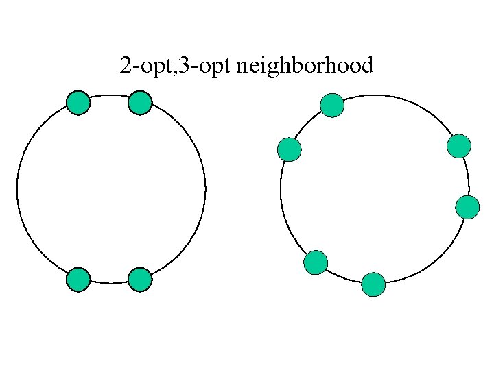
2 -opt, 3 -opt neighborhood

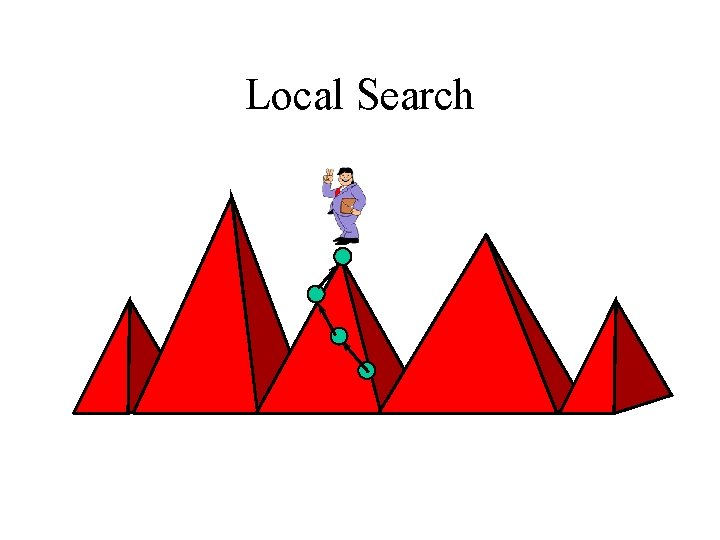
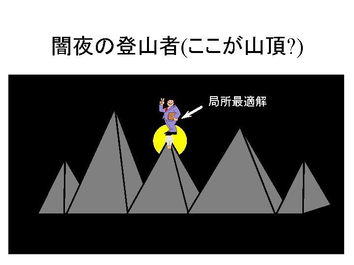
Local Search

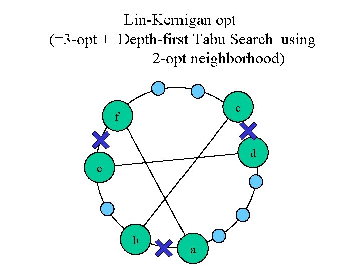
Lin-Kernigan opt (=3 -opt + Depth-first Tabu Search using 2 -opt neighborhood) c f d e b a

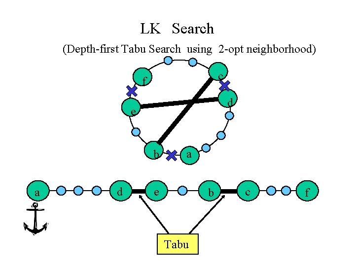
LK Search (Depth-first Tabu Search using 2 -opt neighborhood) c f d e b a d a e b Tabu c f

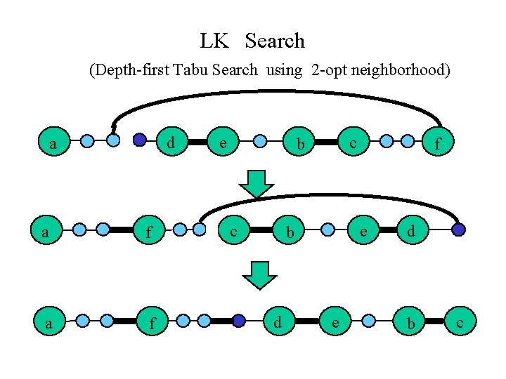
LK Search (Depth-first Tabu Search using 2 -opt neighborhood) d a a f e c b c e b d f e d b c

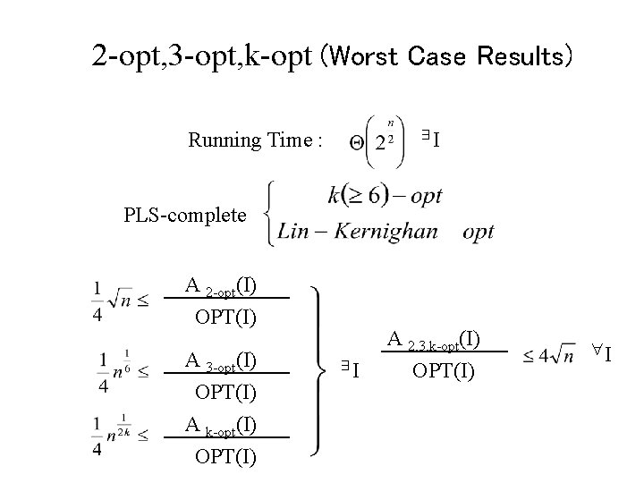
2 -opt, 3 -opt, k-opt (Worst Case Results) Running Time : ∃I PLS-complete A 2 -opt(I) OPT(I) A 3 -opt(I) OPT(I) A k-opt(I) OPT(I) ∃I A 2, 3, k-opt(I) OPT(I) ∀I

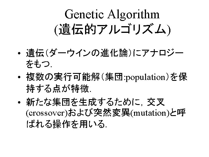
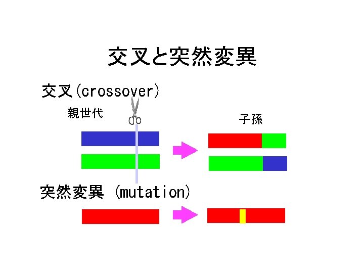
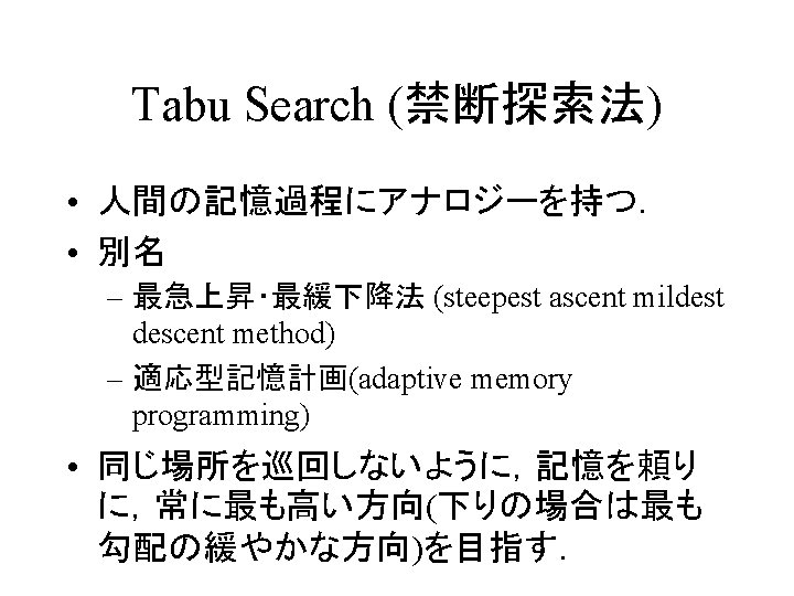
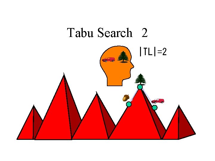
Tabu Search 2 |TL|=2

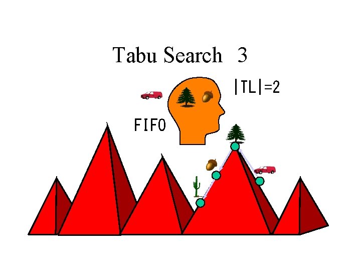
Tabu Search 3 |TL|=2 FIFO

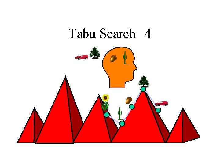
Tabu Search 4

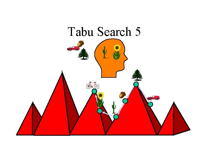
Tabu Search 5

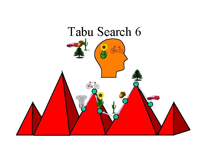
Tabu Search 6

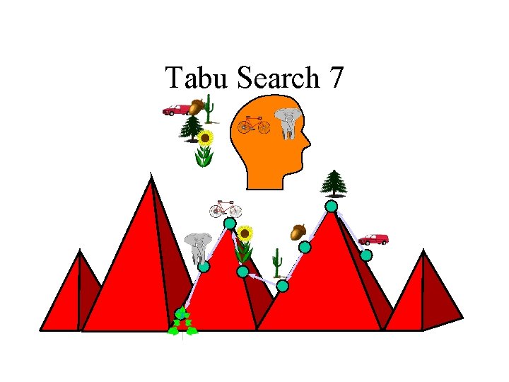
Tabu Search 7

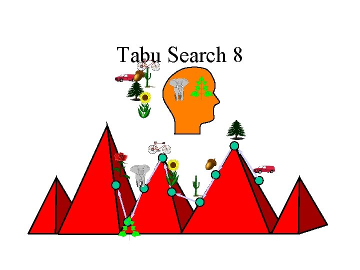
Tabu Search 8

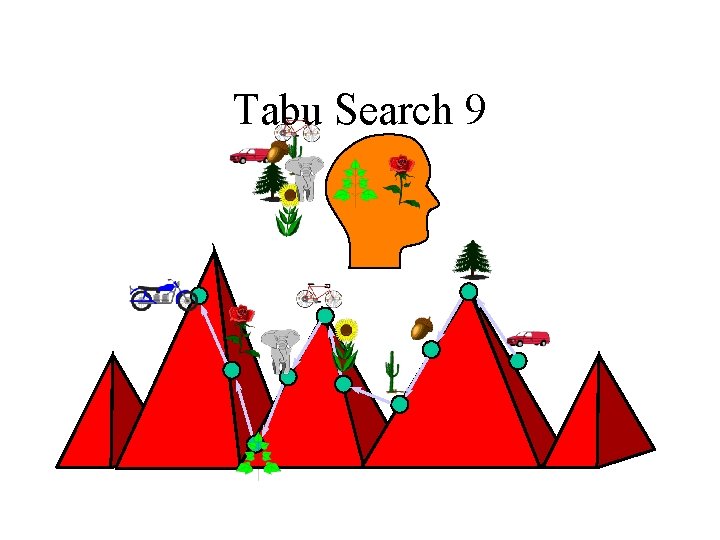
Tabu Search 9

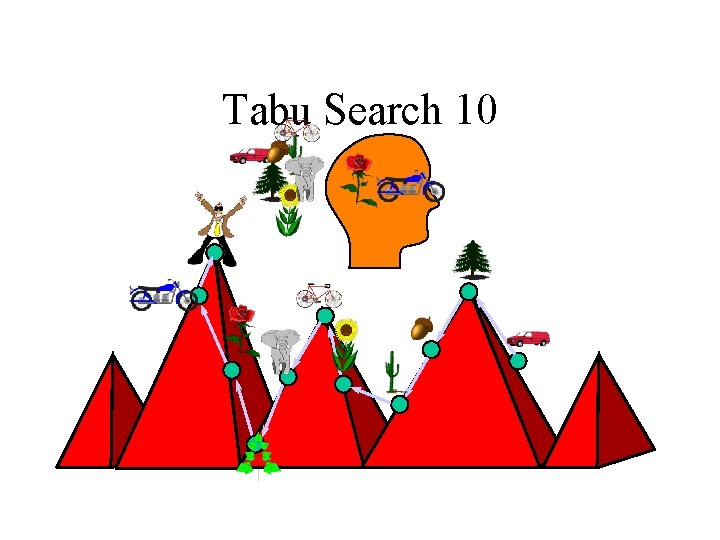
Tabu Search 10