Financial Engineering Zvi Wiener mswienermscc huji ac il

Financial Engineering Zvi Wiener mswiener@mscc. huji. ac. il tel: 02 -588 -3049 Zvi Wiener Cont. Time. Fin - 1 1

Main Books Shimko D. Finance in Continuous Time, A Primer. Kolb Publishing Company, 1992, ISBN 1 -878975 -07 -2 F Wilmott P. , S. Howison, J. Dewynne, The Mathematics of Financial Derivatives, A Student Introduction, Cambridge University Press, 1996, ISBN 0 -521 -49789 -2 F Zvi Wiener Cont. Time. Fin - 1 2

Useful Books Duffie D. , Dynamic Asset Pricing Theory. F Duffie D. , Security Markets, Stochastic Models. F Neftci S. , An Introduction to the Mathematics of Financial Derivatives. F Steele M. , Invitation to Stochastic Differential Equations and Financial Applications. F Karatzas I. , and S. Shreve, BM and Stochastic Calculus. F Zvi Wiener Cont. Time. Fin - 1 3

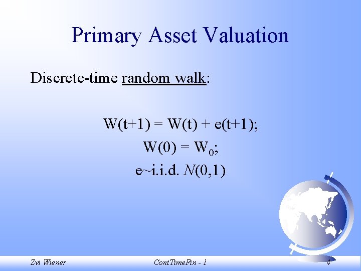
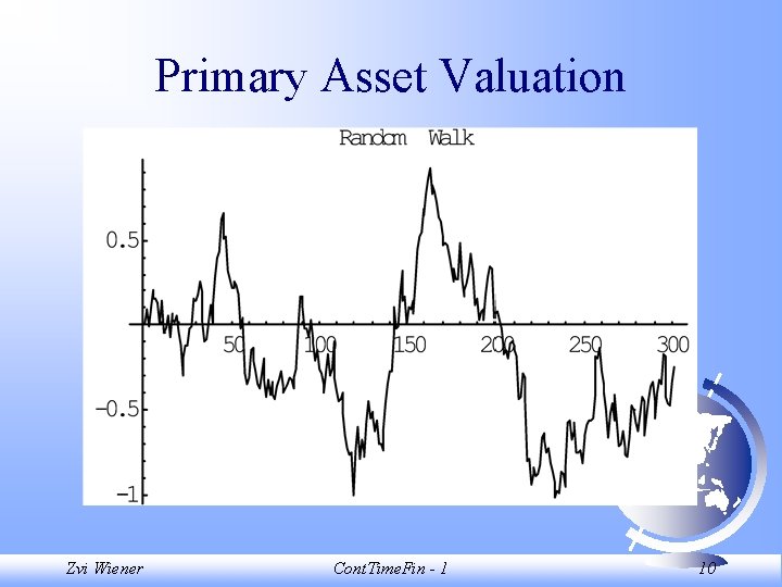
Primary Asset Valuation Discrete-time random walk: W(t+1) = W(t) + e(t+1); W(0) = W 0; e~i. i. d. N(0, 1) Zvi Wiener Cont. Time. Fin - 1 4

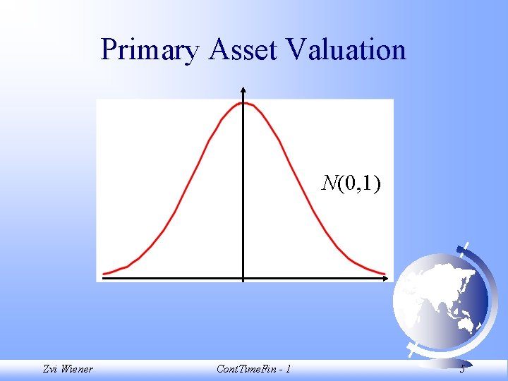
Primary Asset Valuation N(0, 1) Zvi Wiener Cont. Time. Fin - 1 5

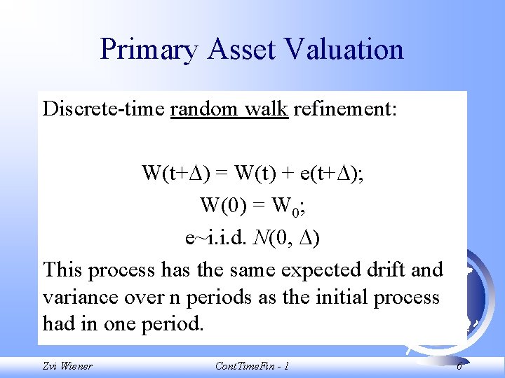
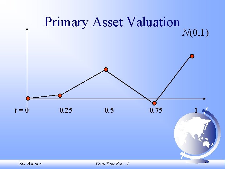
Primary Asset Valuation Discrete-time random walk refinement: W(t+ ) = W(t) + e(t+ ); W(0) = W 0; e~i. i. d. N(0, ) This process has the same expected drift and variance over n periods as the initial process had in one period. Zvi Wiener Cont. Time. Fin - 1 6

Primary Asset Valuation t=0 Zvi Wiener 0. 25 0. 5 Cont. Time. Fin - 1 0. 75 N(0, 1) 1 7

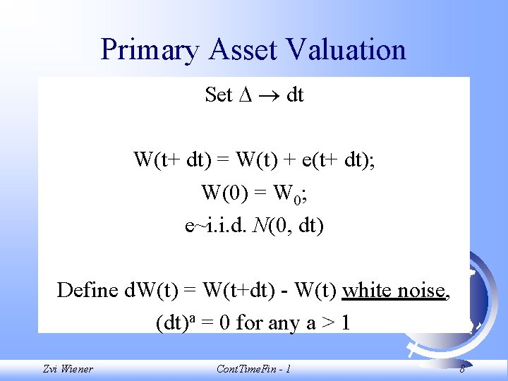
Primary Asset Valuation Set dt W(t+ dt) = W(t) + e(t+ dt); W(0) = W 0; e~i. i. d. N(0, dt) Define d. W(t) = W(t+dt) - W(t) white noise, (dt)a = 0 for any a > 1 Zvi Wiener Cont. Time. Fin - 1 8

Primary Asset Valuation Needs["Statistics`Normal. Distribution`"] nor[mu_, sig_]: =Random[Normal. Distribution[mu, sig]]; tt=Nest. List[ (#+nor[0, 0. 1])&, 0, 300]; List. Plot[tt, Plot. Joined->True, Plot. Label->"Random Walk"]; Zvi Wiener Cont. Time. Fin - 1 9

Primary Asset Valuation Zvi Wiener Cont. Time. Fin - 1 10

Main Properties 1. E[d. W(t)] = 0 2. E[d. W(t) dt] = E[d. W(t)] dt = 0 3. E[d. W(t)2] = dt Zvi Wiener Cont. Time. Fin - 1 11

Main Properties (cont. ) 4. Var[d. W(t)2] = E[d. W(t)4] - E 2[d. W(t)2] = 3 dt 2 - dt 2 = 0 5. E[(d. W(t)dt)2] = E [d. W(t)2] (dt)2 = 0 6. Var[d. W(t)dt] = E[(d. W(t)dt)4] - E 2[d. W(t)dt] = 0 Zvi Wiener Cont. Time. Fin - 1 12

E[d. W(t)] = 0 By definition the mean of the normally distributed variable is zero. Zvi Wiener Cont. Time. Fin - 1 13

E[d. W(t) dt] = E[d. W(t)] dt = 0 The expectation of the product of a random variable (d. W) and a constant (dt) equals the constant times the expected value of the random variable. Zvi Wiener Cont. Time. Fin - 1 14

E[d. W(t)2] = dt For any distribution with zero mean the expected value of the squared random variable is the same as its variance. Zvi Wiener Cont. Time. Fin - 1 15

2 Var[d. W(t) ] 4 E[d. W(t) ] - = 2 2 E [d. W(t) ] = 3 dt 2 - dt 2 = 0 The fourth central moment of the standard normal distribution is 3, and (dt)2 = 0. Zvi Wiener Cont. Time. Fin - 1 16

E[(d. W(t)dt)2] = E [d. W(t)2] (dt)2 = 0 Follows from properties 2 and 3. Zvi Wiener Cont. Time. Fin - 1 17

Var[d. W(t)dt] = 4 2 E[(d. W(t)dt) ] - E [d. W(t)dt] = 0 Follows from properties 2 and 5. Zvi Wiener Cont. Time. Fin - 1 18

Important Property if Var[f(d. W)] = 0 then E[f(d. W)] = f(d. W) Zvi Wiener Cont. Time. Fin - 1 19

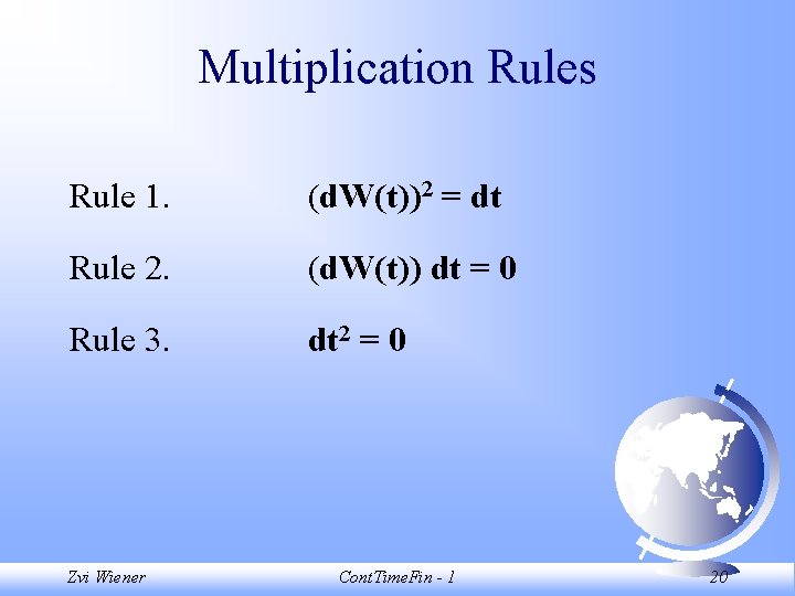
Multiplication Rules Rule 1. (d. W(t))2 = dt Rule 2. (d. W(t)) dt = 0 Rule 3. dt 2 = 0 Zvi Wiener Cont. Time. Fin - 1 20

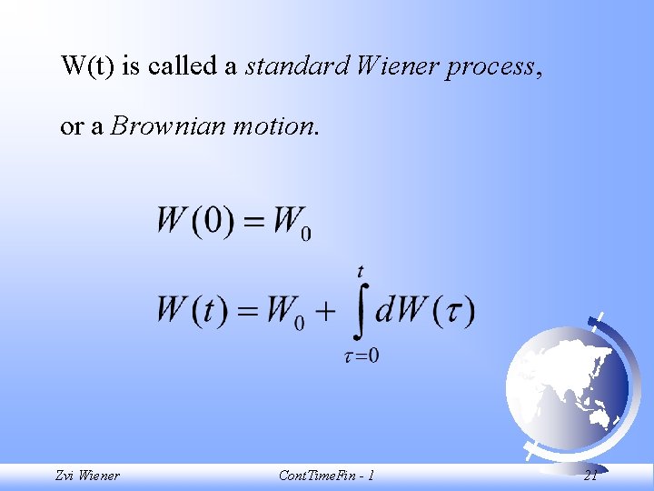
W(t) is called a standard Wiener process, or a Brownian motion. Zvi Wiener Cont. Time. Fin - 1 21

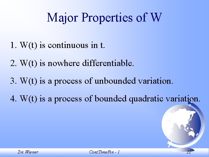
Major Properties of W 1. W(t) is continuous in t. 2. W(t) is nowhere differentiable. 3. W(t) is a process of unbounded variation. 4. W(t) is a process of bounded quadratic variation. Zvi Wiener Cont. Time. Fin - 1 22

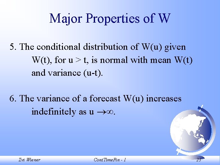
Major Properties of W 5. The conditional distribution of W(u) given W(t), for u > t, is normal with mean W(t) and variance (u-t). 6. The variance of a forecast W(u) increases indefinitely as u . Zvi Wiener Cont. Time. Fin - 1 23

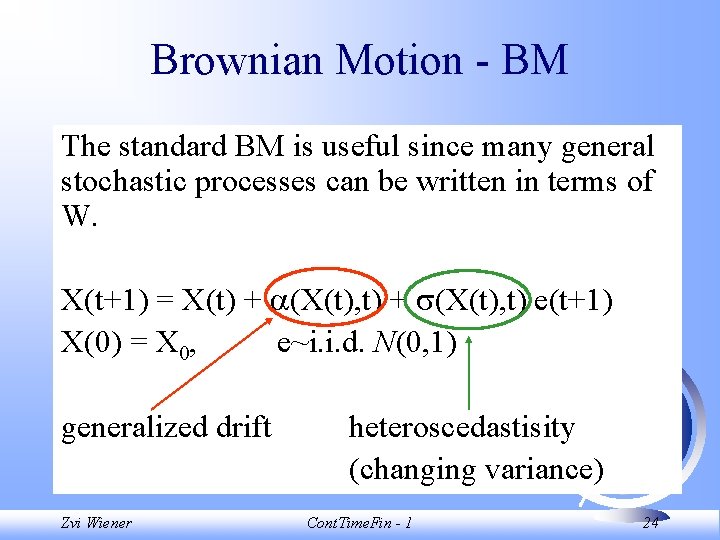
Brownian Motion - BM The standard BM is useful since many general stochastic processes can be written in terms of W. X(t+1) = X(t) + (X(t), t) e(t+1) X(0) = X 0, e~i. i. d. N(0, 1) generalized drift Zvi Wiener heteroscedastisity (changing variance) Cont. Time. Fin - 1 24

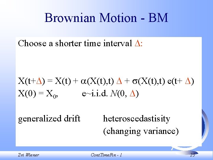
Brownian Motion - BM Choose a shorter time interval : X(t+ ) = X(t) + (X(t), t) e(t+ ) X(0) = X 0, e~i. i. d. N(0, ) generalized drift Zvi Wiener heteroscedastisity (changing variance) Cont. Time. Fin - 1 25

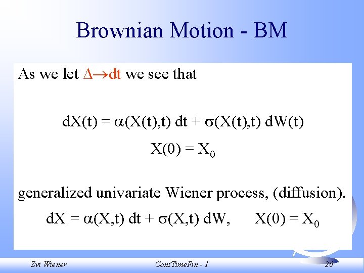
Brownian Motion - BM As we let dt we see that d. X(t) = (X(t), t) dt + (X(t), t) d. W(t) X(0) = X 0 generalized univariate Wiener process, (diffusion). d. X = (X, t) dt + (X, t) d. W, Zvi Wiener Cont. Time. Fin - 1 X(0) = X 0 26

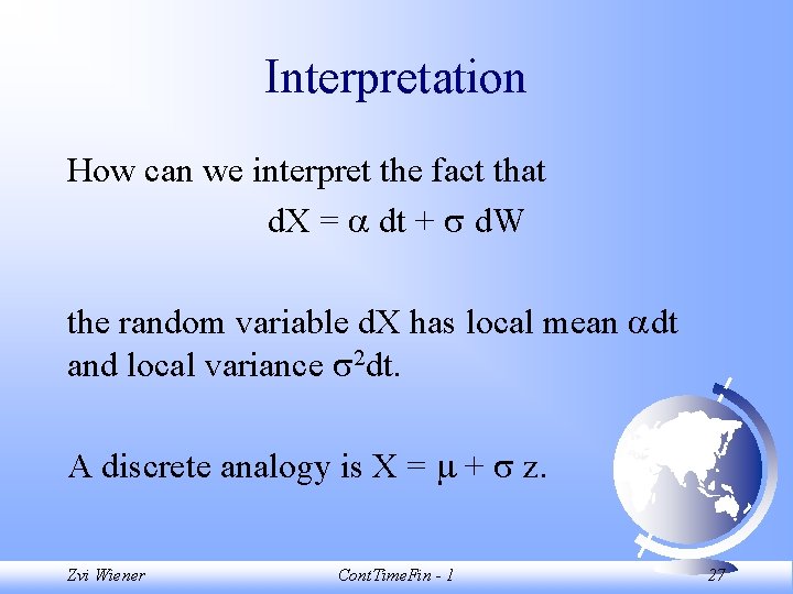
Interpretation How can we interpret the fact that d. X = dt + d. W the random variable d. X has local mean dt and local variance 2 dt. A discrete analogy is X = + z. Zvi Wiener Cont. Time. Fin - 1 27

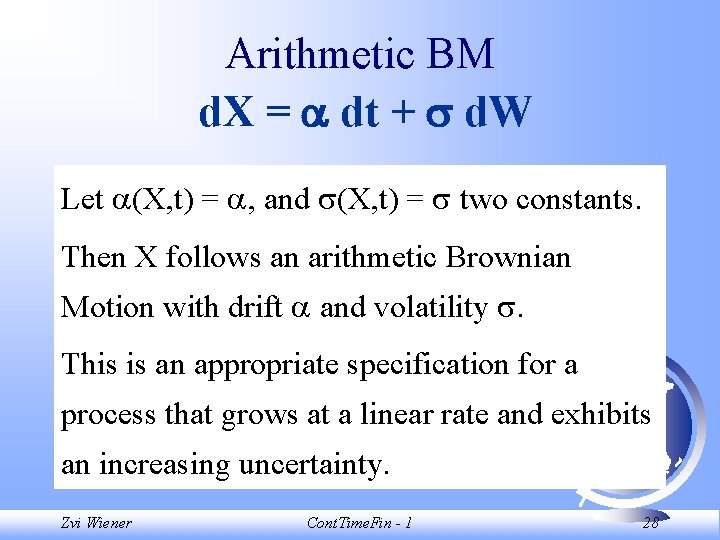
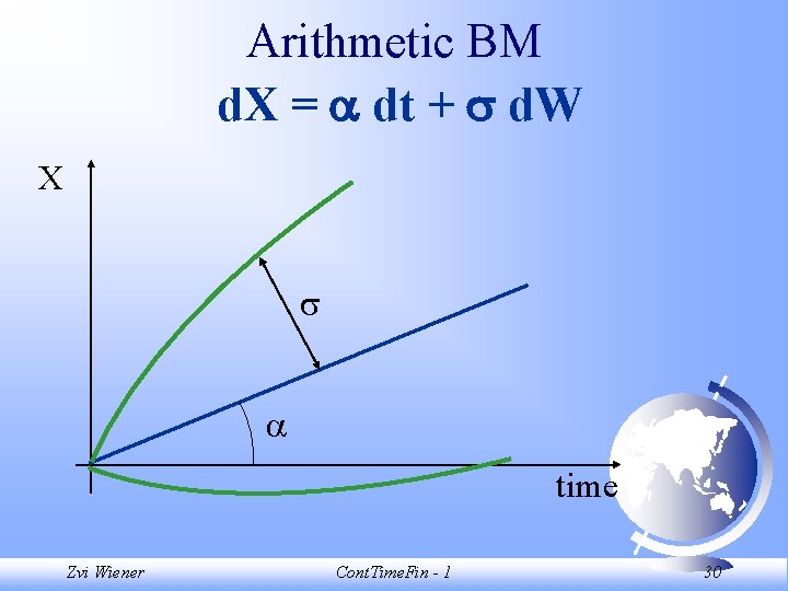
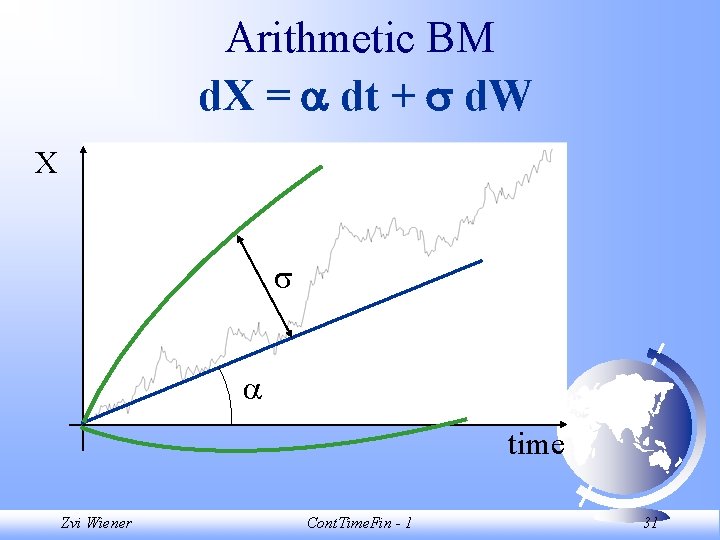
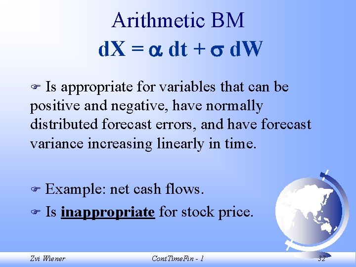
Arithmetic BM d. X = dt + d. W Let (X, t) = , and (X, t) = two constants. Then X follows an arithmetic Brownian Motion with drift and volatility . This is an appropriate specification for a process that grows at a linear rate and exhibits an increasing uncertainty. Zvi Wiener Cont. Time. Fin - 1 28

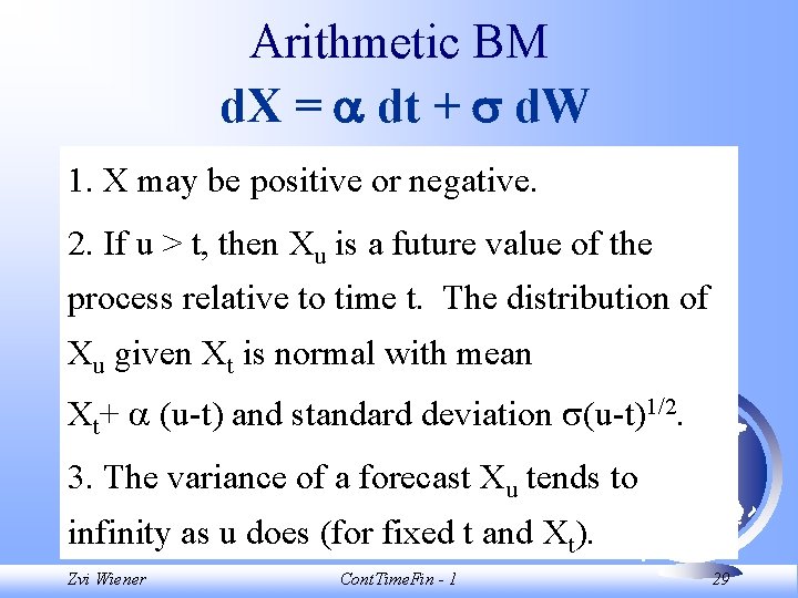
Arithmetic BM d. X = dt + d. W 1. X may be positive or negative. 2. If u > t, then Xu is a future value of the process relative to time t. The distribution of Xu given Xt is normal with mean Xt+ (u-t) and standard deviation (u-t)1/2. 3. The variance of a forecast Xu tends to infinity as u does (for fixed t and Xt). Zvi Wiener Cont. Time. Fin - 1 29

Arithmetic BM d. X = dt + d. W X time Zvi Wiener Cont. Time. Fin - 1 30

Arithmetic BM d. X = dt + d. W X time Zvi Wiener Cont. Time. Fin - 1 31

Arithmetic BM d. X = dt + d. W Is appropriate for variables that can be positive and negative, have normally distributed forecast errors, and have forecast variance increasing linearly in time. F Example: net cash flows. F Is inappropriate for stock price. F Zvi Wiener Cont. Time. Fin - 1 32

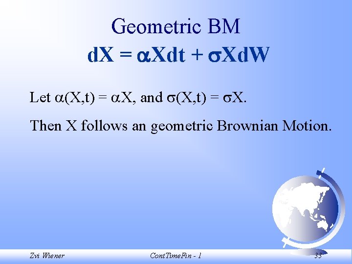
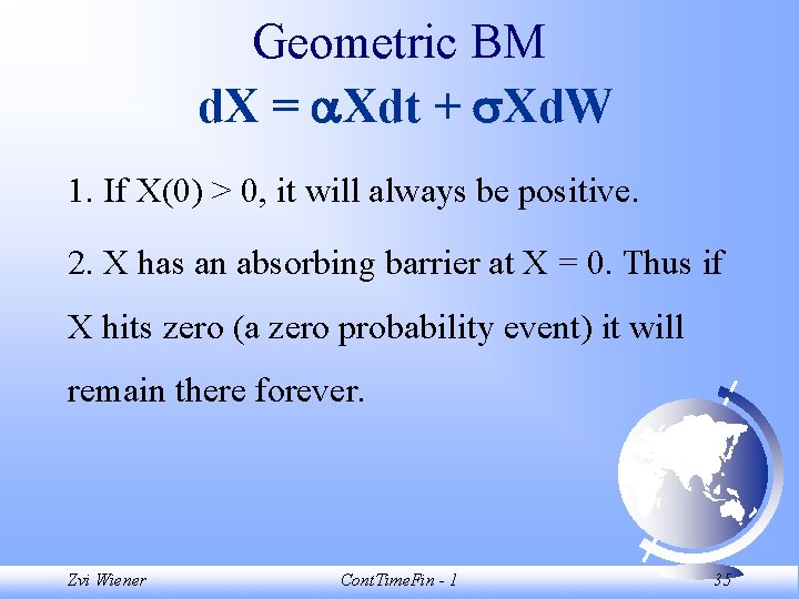
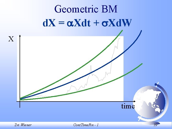
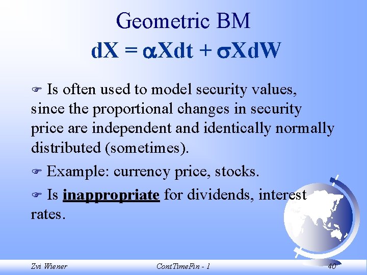
Geometric BM d. X = Xdt + Xd. W Let (X, t) = X, and (X, t) = X. Then X follows an geometric Brownian Motion. Zvi Wiener Cont. Time. Fin - 1 33

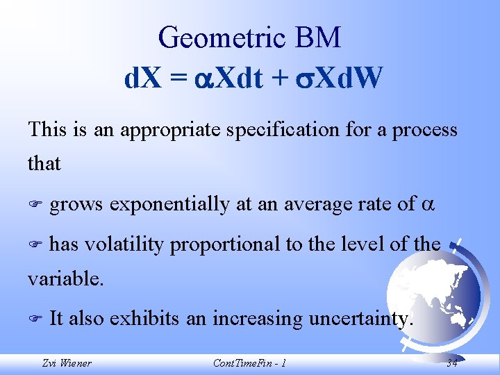
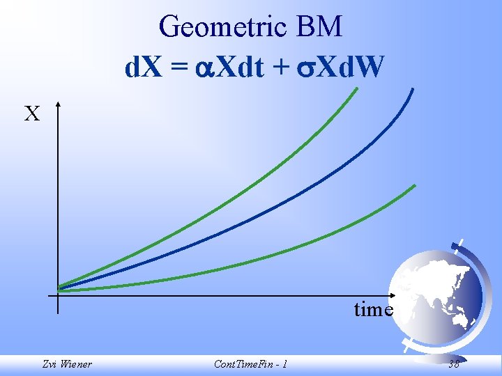
Geometric BM d. X = Xdt + Xd. W This is an appropriate specification for a process that F grows exponentially at an average rate of F has volatility proportional to the level of the variable. F It also exhibits an increasing uncertainty. Zvi Wiener Cont. Time. Fin - 1 34

Geometric BM d. X = Xdt + Xd. W 1. If X(0) > 0, it will always be positive. 2. X has an absorbing barrier at X = 0. Thus if X hits zero (a zero probability event) it will remain there forever. Zvi Wiener Cont. Time. Fin - 1 35

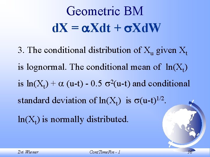
Geometric BM d. X = Xdt + Xd. W 3. The conditional distribution of Xu given Xt is lognormal. The conditional mean of ln(Xt) is ln(Xt) + (u-t) - 0. 5 2(u-t) and conditional standard deviation of ln(Xt) is (u-t)1/2. ln(Xt) is normally distributed. Zvi Wiener Cont. Time. Fin - 1 36

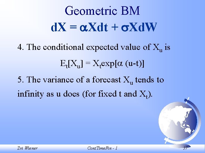
Geometric BM d. X = Xdt + Xd. W 4. The conditional expected value of Xu is Et[Xu] = Xtexp[ (u-t)] 5. The variance of a forecast Xu tends to infinity as u does (for fixed t and Xt). Zvi Wiener Cont. Time. Fin - 1 37

Geometric BM d. X = Xdt + Xd. W X time Zvi Wiener Cont. Time. Fin - 1 38

Geometric BM d. X = Xdt + Xd. W X time Zvi Wiener Cont. Time. Fin - 1 39

Geometric BM d. X = Xdt + Xd. W Is often used to model security values, since the proportional changes in security price are independent and identically normally distributed (sometimes). F Example: currency price, stocks. F Is inappropriate for dividends, interest rates. F Zvi Wiener Cont. Time. Fin - 1 40

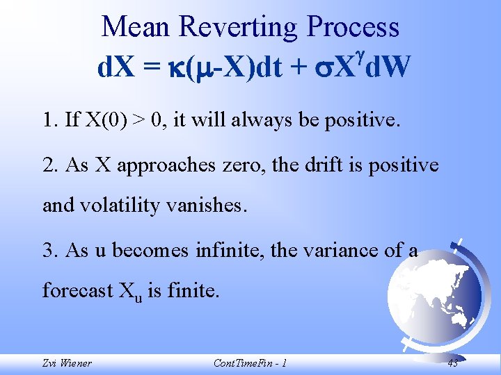
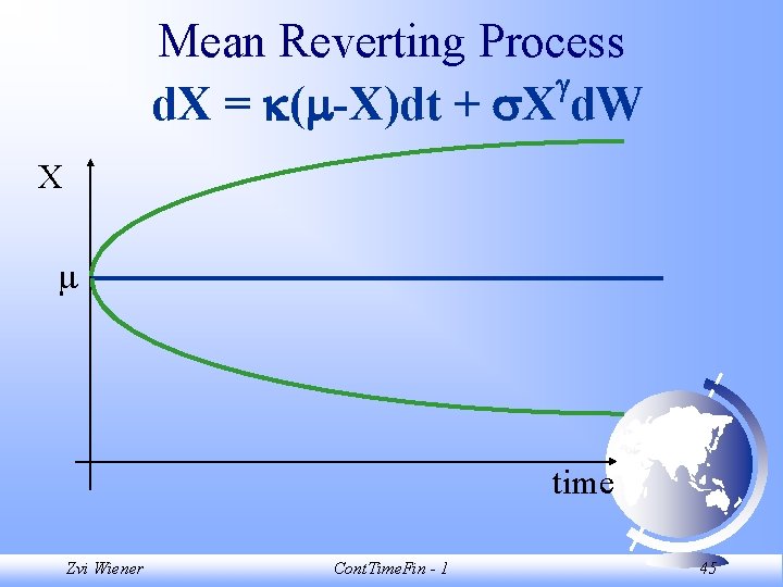
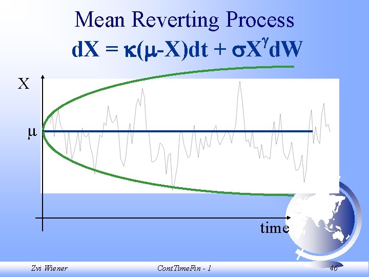
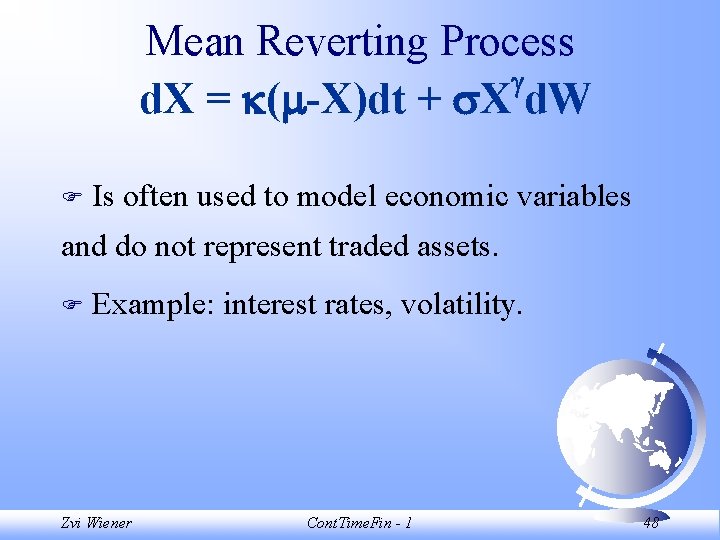
Mean Reverting Process d. X = ( -X)dt + X d. W Ornstein-Uhlenbeck when = 1 Let (X, t) = ( -X), and (X, t) = X , where 0 - speed of adjustment - long run mean - volatility Zvi Wiener Cont. Time. Fin - 1 41

Mean Reverting Process d. X = ( -X)dt + X d. W This is an appropriate specification for a process that has a long run value but may be beset by short -term disturbances. We assume that , , and are positive for simplicity. Zvi Wiener Cont. Time. Fin - 1 42

Mean Reverting Process d. X = ( -X)dt + X d. W 1. If X(0) > 0, it will always be positive. 2. As X approaches zero, the drift is positive and volatility vanishes. 3. As u becomes infinite, the variance of a forecast Xu is finite. Zvi Wiener Cont. Time. Fin - 1 43

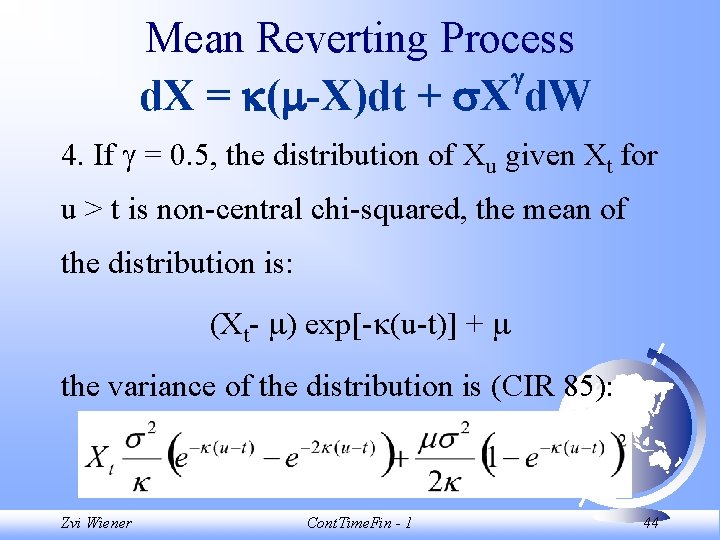
Mean Reverting Process d. X = ( -X)dt + X d. W 4. If = 0. 5, the distribution of Xu given Xt for u > t is non-central chi-squared, the mean of the distribution is: (Xt- ) exp[- (u-t)] + the variance of the distribution is (CIR 85): Zvi Wiener Cont. Time. Fin - 1 44

Mean Reverting Process d. X = ( -X)dt + X d. W X time Zvi Wiener Cont. Time. Fin - 1 45

Mean Reverting Process d. X = ( -X)dt + X d. W X time Zvi Wiener Cont. Time. Fin - 1 46

Mean Reverting Process d. X = ( -X)dt + X d. W Seed. Random[2] tt=Nest. List[ (#+0. 3(1 -#)+0. 1*#*nor[0, 0. 1])&, 1. 01, 130]; List. Plot[tt, Plot. Joined->True, Axes->False]; Zvi Wiener Cont. Time. Fin - 1 47

Mean Reverting Process d. X = ( -X)dt + X d. W F Is often used to model economic variables and do not represent traded assets. F Example: interest rates, volatility. Zvi Wiener Cont. Time. Fin - 1 48

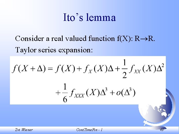
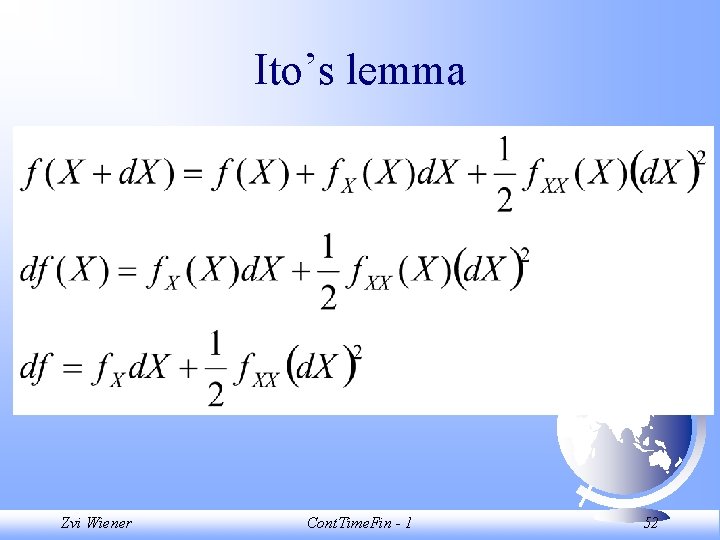
Ito’s lemma Consider a real valued function f(X): R R. Taylor series expansion: Zvi Wiener Cont. Time. Fin - 1 49

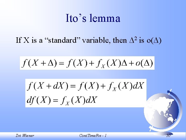
Ito’s lemma If X is a “standard” variable, then 2 is o( ) Zvi Wiener Cont. Time. Fin - 1 50

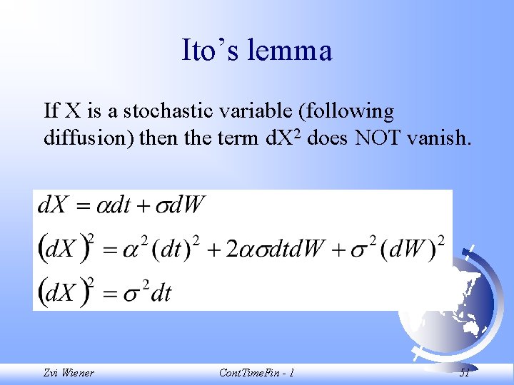
Ito’s lemma If X is a stochastic variable (following diffusion) then the term d. X 2 does NOT vanish. Zvi Wiener Cont. Time. Fin - 1 51

Ito’s lemma Zvi Wiener Cont. Time. Fin - 1 52

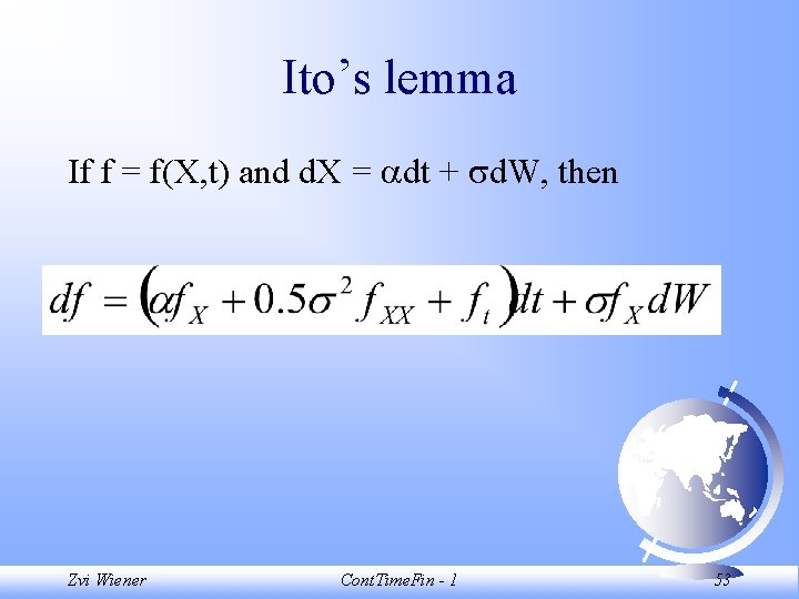
Ito’s lemma If f = f(X, t) and d. X = dt + d. W, then Zvi Wiener Cont. Time. Fin - 1 53

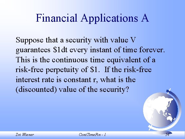
Financial Applications A Suppose that a security with value V guarantees $1 dt every instant of time forever. This is the continuous time equivalent of a risk-free perpetuity of $1. If the risk-free interest rate is constant r, what is the (discounted) value of the security? Zvi Wiener Cont. Time. Fin - 1 54

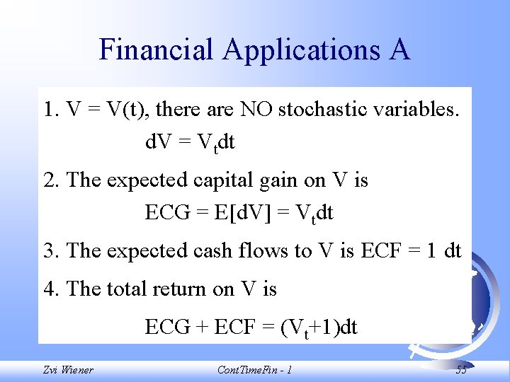
Financial Applications A 1. V = V(t), there are NO stochastic variables. d. V = Vtdt 2. The expected capital gain on V is ECG = E[d. V] = Vtdt 3. The expected cash flows to V is ECF = 1 dt 4. The total return on V is ECG + ECF = (Vt+1)dt Zvi Wiener Cont. Time. Fin - 1 55

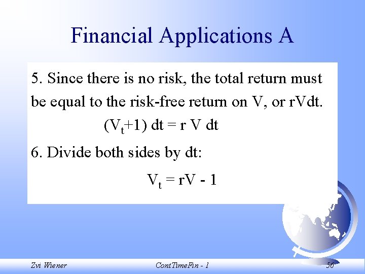
Financial Applications A 5. Since there is no risk, the total return must be equal to the risk-free return on V, or r. Vdt. (Vt+1) dt = r V dt 6. Divide both sides by dt: Vt = r. V - 1 Zvi Wiener Cont. Time. Fin - 1 56

Financial Applications A Vt = r. V - 1 DSolve[ V'[t]==r*V[t]-1, V[t], t ] V(t) = c Exp[r t] + 1/r given V(0) one can find c Zvi Wiener Cont. Time. Fin - 1 57

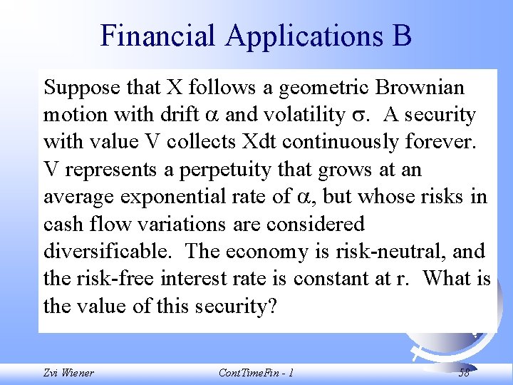
Financial Applications B Suppose that X follows a geometric Brownian motion with drift and volatility . A security with value V collects Xdt continuously forever. V represents a perpetuity that grows at an average exponential rate of , but whose risks in cash flow variations are considered diversificable. The economy is risk-neutral, and the risk-free interest rate is constant at r. What is the value of this security? Zvi Wiener Cont. Time. Fin - 1 58

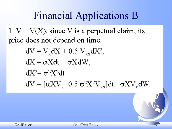
Financial Applications B 1. V = V(X), since V is a perpetual claim, its price does not depend on time. d. V = Vxd. X + 0. 5 Vxxd. X 2, d. X = Xdt + Xd. W, d. X 2= 2 X 2 dt d. V = [ XVx+0. 5 2 X 2 Vxx]dt + XVxd. W Zvi Wiener Cont. Time. Fin - 1 59

Financial Applications B 2. The expected capital gain: ECG = E[d. V] = [ XVx+0. 5 2 X 2 Vxx]dt since E[d. W] = 0 3. The Expected cash flow: ECF = X dt Zvi Wiener Cont. Time. Fin - 1 60

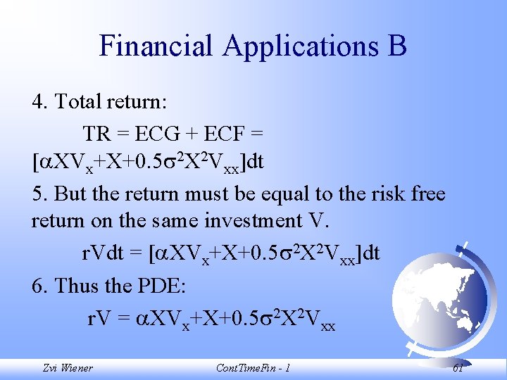
Financial Applications B 4. Total return: TR = ECG + ECF = [ XVx+X+0. 5 2 X 2 Vxx]dt 5. But the return must be equal to the risk free return on the same investment V. r. Vdt = [ XVx+X+0. 5 2 X 2 Vxx]dt 6. Thus the PDE: r. V = XVx+X+0. 5 2 X 2 Vxx Zvi Wiener Cont. Time. Fin - 1 61

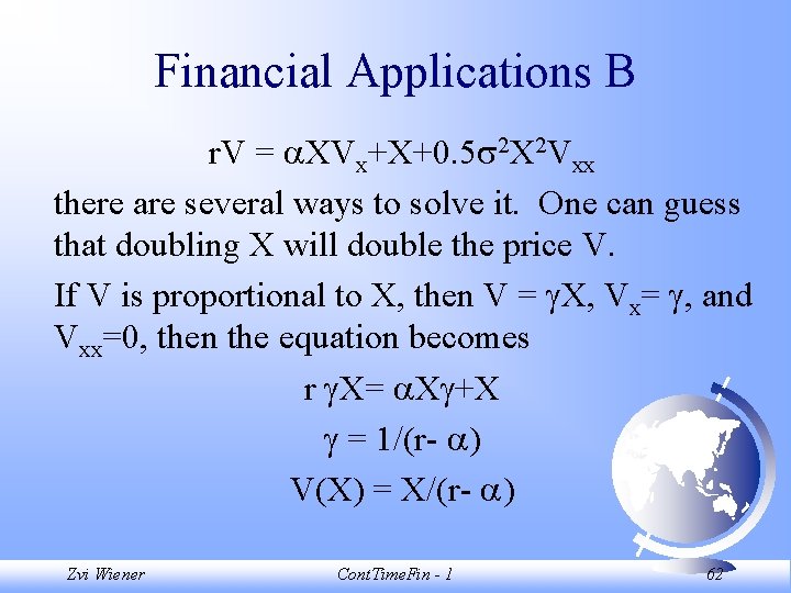
Financial Applications B r. V = XVx+X+0. 5 2 X 2 Vxx there are several ways to solve it. One can guess that doubling X will double the price V. If V is proportional to X, then V = X, Vx= , and Vxx=0, then the equation becomes r X= X +X = 1/(r- ) V(X) = X/(r- ) Zvi Wiener Cont. Time. Fin - 1 62