Faculty of Engineering Mechanical Engineering Department MATH 2140

Faculty of Engineering Mechanical Engineering Department MATH 2140 Numerical Methods Instructor: Dr. Mohamed El-Shazly Associate Prof. of Mechanical Design and Tribology melshazly@ksu. edu. sa Office: F 072 1

Curve-Fitting Polynomial Interpolation 2

Outline n Introduction n Curve Fitting? n Interpolation? 3

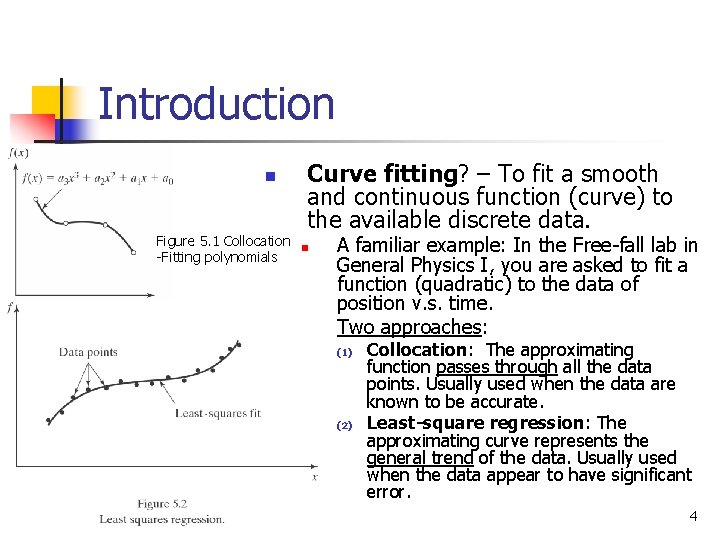
Introduction n Curve fitting? – To fit a smooth and continuous function (curve) to the available discrete data. Figure 5. 1 Collocation n -Fitting polynomials n A familiar example: In the Free-fall lab in General Physics I, you are asked to fit a function (quadratic) to the data of position v. s. time. Two approaches: (1) (2) Collocation: The approximating function passes through all the data points. Usually used when the data are known to be accurate. Least-square regression: The approximating curve represents the general trend of the data. Usually used when the data appear to have significant error. 4

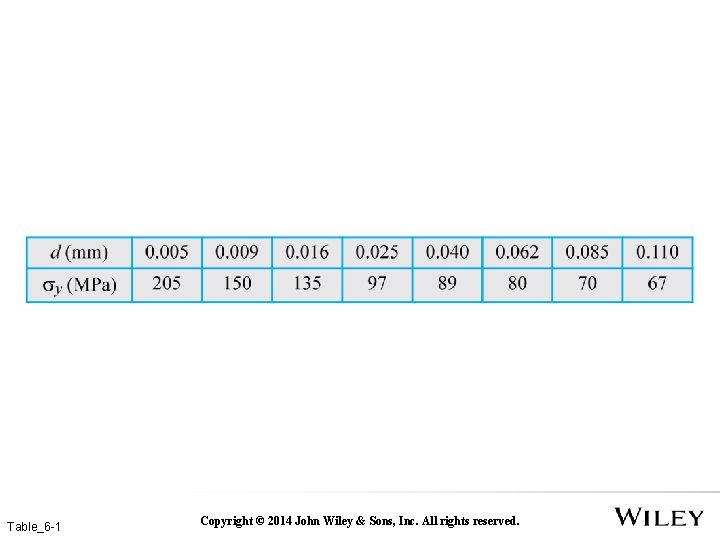
Table_6 -1 Copyright © 2014 John Wiley & Sons, Inc. All rights reserved.

Fig_6 -1 Copyright © 2014 John Wiley & Sons, Inc. All rights reserved.

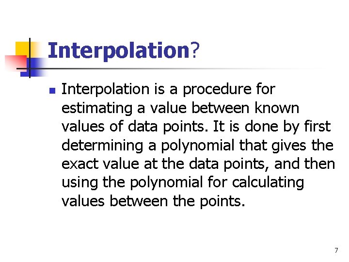
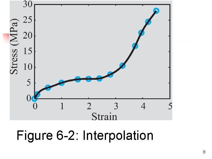
Interpolation? n Interpolation is a procedure for estimating a value between known values of data points. It is done by first determining a polynomial that gives the exact value at the data points, and then using the polynomial for calculating values between the points. 7

Fig_6 -2 Figure 6 -2: Interpolation 8

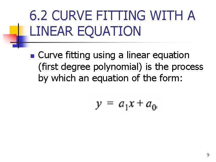
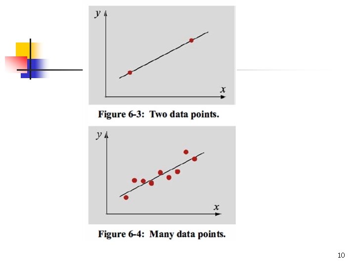
6. 2 CURVE FITTING WITH A LINEAR EQUATION n Curve fitting using a linear equation (first degree polynomial) is the process by which an equation of the form: 9

10

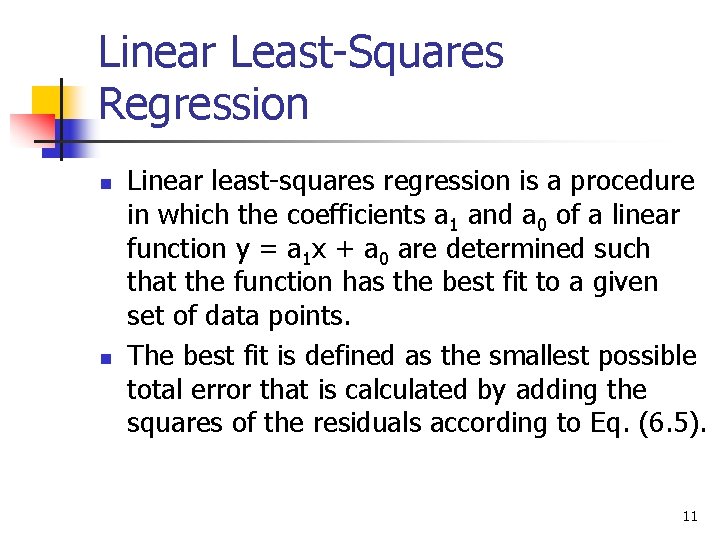
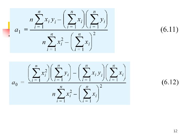
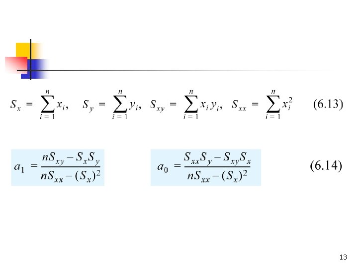
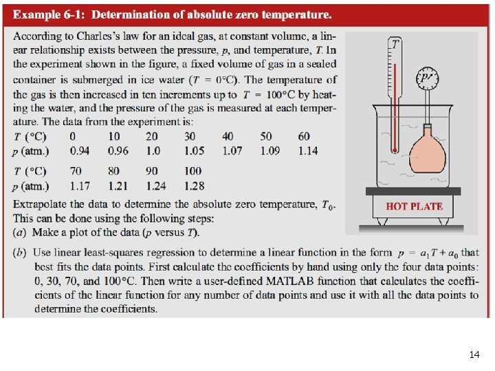
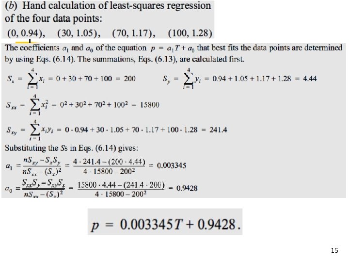
Linear Least-Squares Regression n n Linear least-squares regression is a procedure in which the coefficients a 1 and a 0 of a linear function y = a 1 x + a 0 are determined such that the function has the best fit to a given set of data points. The best fit is defined as the smallest possible total error that is calculated by adding the squares of the residuals according to Eq. (6. 5). 11

12

13

14

15

Curve Fitting Regression Linear Regression Polynomial Regression Multiple Linear Regression Non-linear Regression Interpolation Newton's Divided-Difference Interpolation Lagrange Interpolating Polynomials Spline Interpolation 16

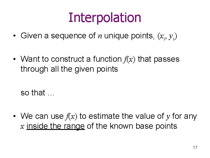
Interpolation • Given a sequence of n unique points, (xi, yi) • Want to construct a function f(x) that passes through all the given points so that … • We can use f(x) to estimate the value of y for any x inside the range of the known base points 17

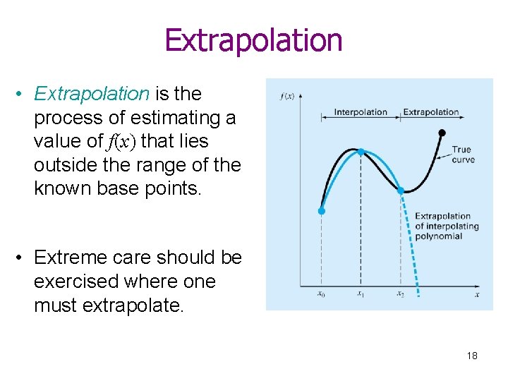
Extrapolation • Extrapolation is the process of estimating a value of f(x) that lies outside the range of the known base points. • Extreme care should be exercised where one must extrapolate. 18

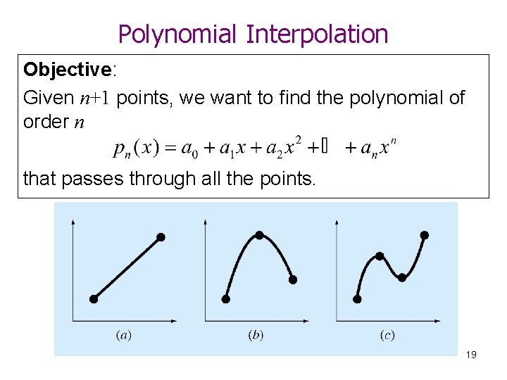
Polynomial Interpolation Objective: Given n+1 points, we want to find the polynomial of order n that passes through all the points. 19

Polynomial Interpolation • The nth-order polynomial that passes through n+1 points is unique, but it can be written in different mathematical formats: – The conventional form – The Newton Form – The Lagrange Form • Useful characteristics of polynomials – Infinitely differentiable – Can be easily integrated – Easy to evaluate 20

Characteristics of Polynomials • Polynomials of order n – Has at most n-1 turning points (local optima) – Hast at most n real roots • At most n different x's that makes pn(x) = 0 • pn(x) passes through x-axis at most n times. • Linear combination of polynomials of order ≤ n results in a polynomial of order ≤ n. – We can express a polynomial as sum of polynomials. 21

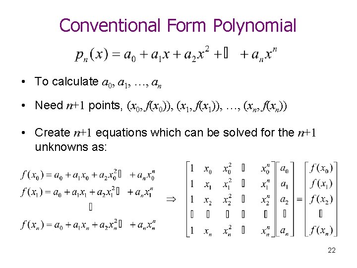
Conventional Form Polynomial • To calculate a 0, a 1, …, an • Need n+1 points, (x 0, f(x 0)), (x 1, f(x 1)), …, (xn, f(xn)) • Create n+1 equations which can be solved for the n+1 unknowns as: 22

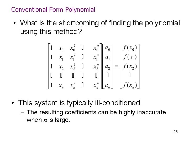
Conventional Form Polynomial • What is the shortcoming of finding the polynomial using this method? • This system is typically ill-conditioned. – The resulting coefficients can be highly inaccurate when n is large. 23

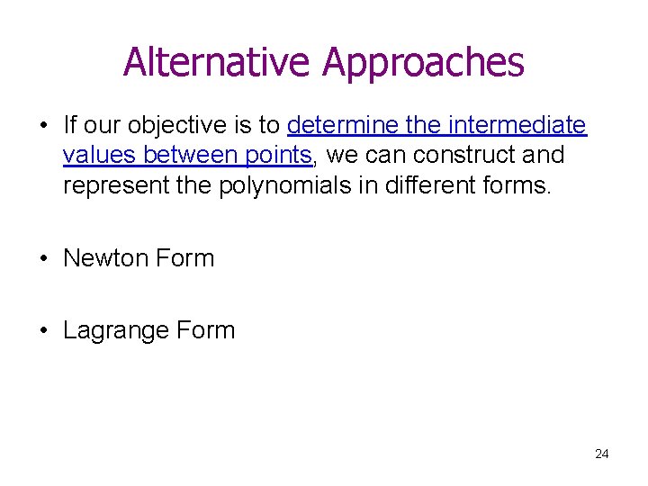
Alternative Approaches • If our objective is to determine the intermediate values between points, we can construct and represent the polynomials in different forms. • Newton Form • Lagrange Form 24

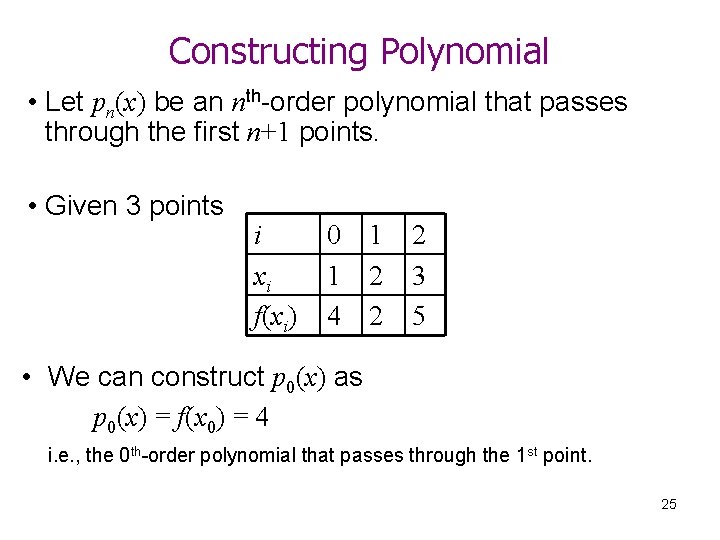
Constructing Polynomial • Let pn(x) be an nth-order polynomial that passes through the first n+1 points. • Given 3 points i xi f(xi) 0 1 4 1 2 2 2 3 5 • We can construct p 0(x) as p 0(x) = f(x 0) = 4 i. e. , the 0 th-order polynomial that passes through the 1 st point. 25

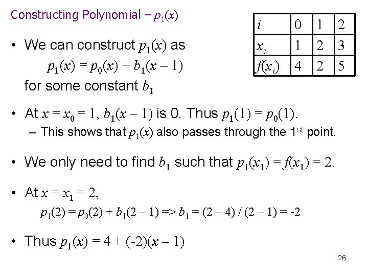
Constructing Polynomial – p 1(x) • We can construct p 1(x) as p 1(x) = p 0(x) + b 1(x – 1) for some constant b 1 i xi f(xi) 0 1 4 1 2 2 2 3 5 • At x = x 0 = 1, b 1(x – 1) is 0. Thus p 1(1) = p 0(1). – This shows that p 1(x) also passes through the 1 st point. • We only need to find b 1 such that p 1(x 1) = f(x 1) = 2. • At x = x 1 = 2, p 1(2) = p 0(2) + b 1(2 – 1) => b 1 = (2 – 4) / (2 – 1) = -2 • Thus p 1(x) = 4 + (-2)(x – 1) 26

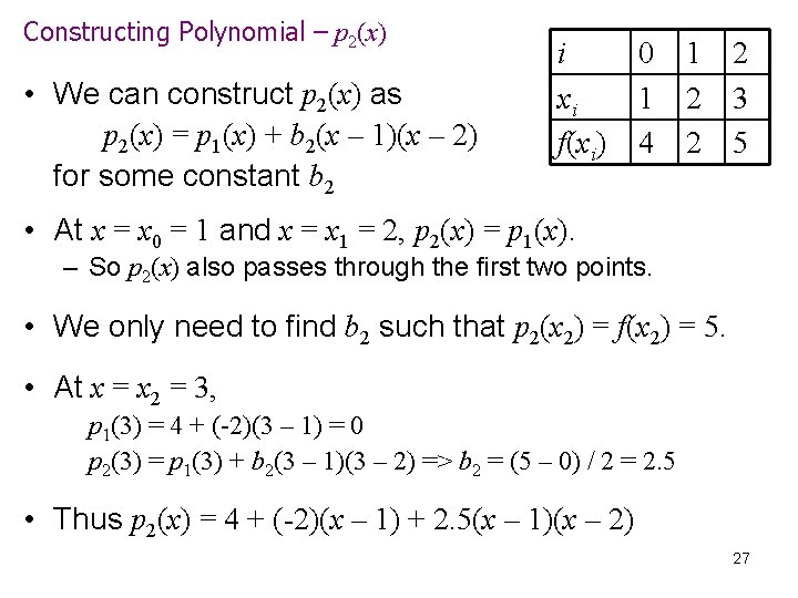
Constructing Polynomial – p 2(x) • We can construct p 2(x) as p 2(x) = p 1(x) + b 2(x – 1)(x – 2) for some constant b 2 i xi f(xi) 0 1 4 1 2 2 2 3 5 • At x = x 0 = 1 and x = x 1 = 2, p 2(x) = p 1(x). – So p 2(x) also passes through the first two points. • We only need to find b 2 such that p 2(x 2) = f(x 2) = 5. • At x = x 2 = 3, p 1(3) = 4 + (-2)(3 – 1) = 0 p 2(3) = p 1(3) + b 2(3 – 1)(3 – 2) => b 2 = (5 – 0) / 2 = 2. 5 • Thus p 2(x) = 4 + (-2)(x – 1) + 2. 5(x – 1)(x – 2) 27

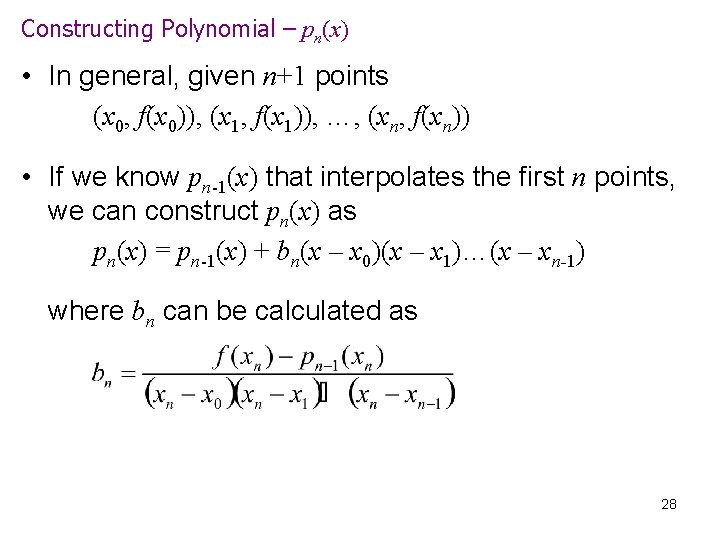
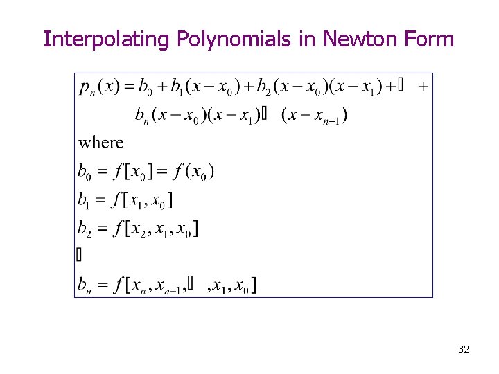
Constructing Polynomial – pn(x) • In general, given n+1 points (x 0, f(x 0)), (x 1, f(x 1)), …, (xn, f(xn)) • If we know pn-1(x) that interpolates the first n points, we can construct pn(x) as pn(x) = pn-1(x) + bn(x – x 0)(x – x 1)…(x – xn-1) where bn can be calculated as 28

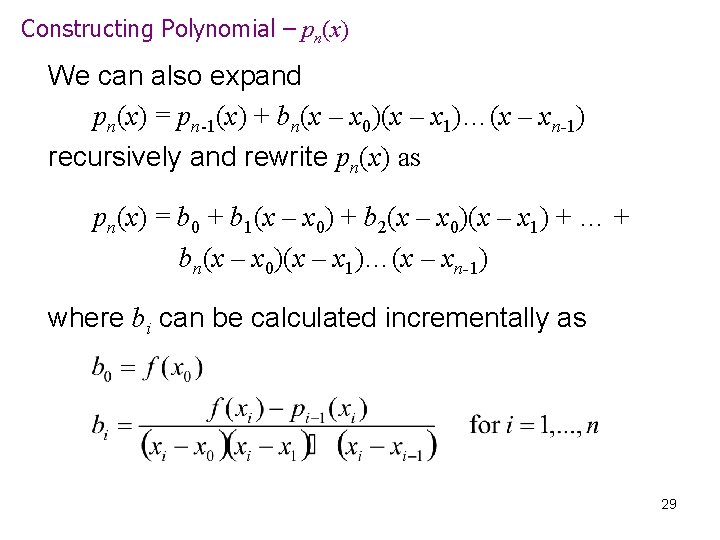
Constructing Polynomial – pn(x) We can also expand pn(x) = pn-1(x) + bn(x – x 0)(x – x 1)…(x – xn-1) recursively and rewrite pn(x) as pn(x) = b 0 + b 1(x – x 0) + b 2(x – x 0)(x – x 1) + … + bn(x – x 0)(x – x 1)…(x – xn-1) where bi can be calculated incrementally as 29

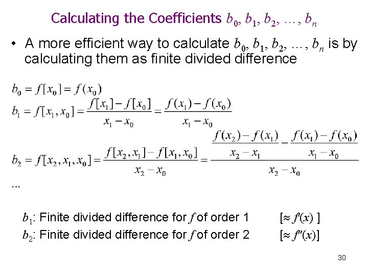
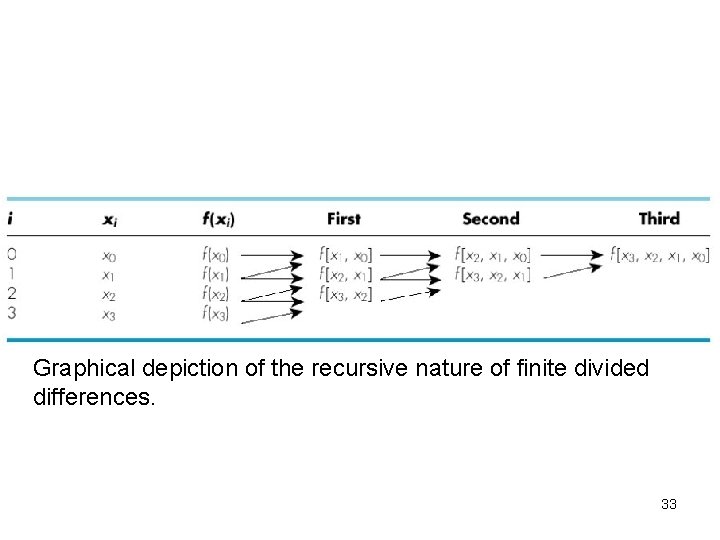
Calculating the Coefficients b 0, b 1, b 2, …, bn • A more efficient way to calculate b 0, b 1, b 2, …, bn is by calculating them as finite divided difference b 1: Finite divided difference for f of order 1 b 2: Finite divided difference for f of order 2 [ f'(x) ] [ f"(x)] 30

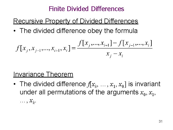
Finite Divided Differences Recursive Property of Divided Differences • The divided difference obey the formula Invariance Theorem • The divided difference f[xk, …, x 1, x 0] is invariant under all permutations of the arguments x 0, x 1, …, xk. 31

Interpolating Polynomials in Newton Form 32

Graphical depiction of the recursive nature of finite divided differences. 33

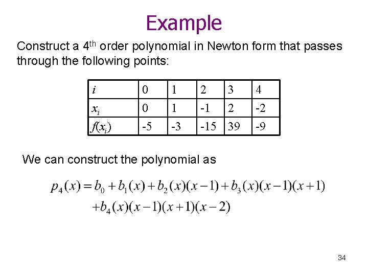
Example Construct a 4 th order polynomial in Newton form that passes through the following points: i xi f(xi) 0 0 -5 1 1 -3 2 3 -1 2 -15 39 4 -2 -9 We can construct the polynomial as 34

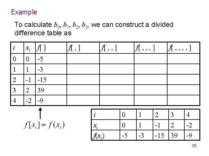
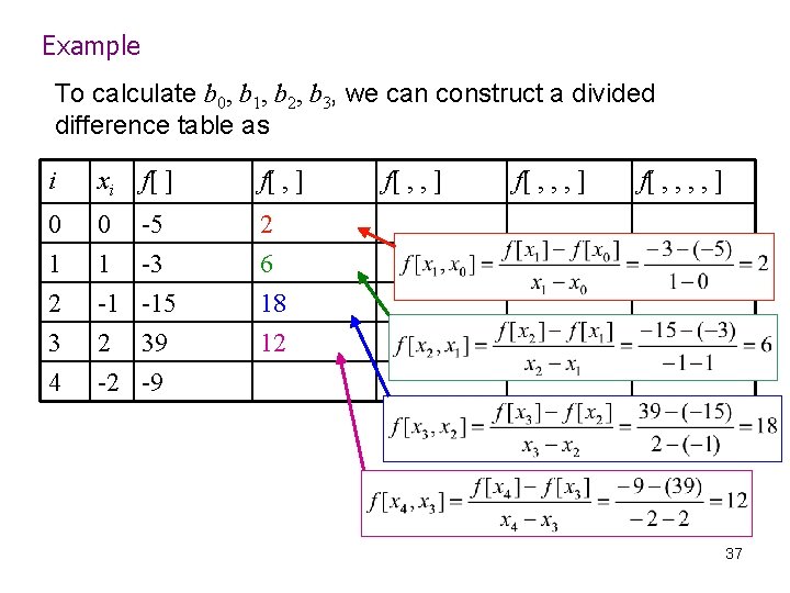
Example To calculate b 0, b 1, b 2, b 3, we can construct a divided difference table as i xi f[ ] 0 1 2 0 -5 1 -3 -1 -15 3 4 2 39 -2 -9 f[ , ] f[ , , ] i xi f(xi) f[ , , , ] 0 0 -5 1 1 -3 f[ , , ] 2 3 -1 2 -15 39 4 -2 -9 35

Example (Exercise) Calculate f[x 1, x 0] and f[x 4, x 3]. i xi f[ ] f[ , , , ] 0 0 -5 1 2 3 4 1 -1 2 -2 -3 f[x 2, x 1] f[x 3, x 2, x 1] f[x 4, x 3, x 2, x 1] -15 f[x 3, x 2] f[x 4, x 3, x 2] 39 f[x 4, x 3] -9 f[ , , ] f[x 1, x 0] f[x 2, x 1, x 0] f[x 3, x 2, x 1, x 0] f[x 4, x 3, x 2, x 1, x 0] 36

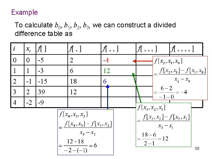
Example To calculate b 0, b 1, b 2, b 3, we can construct a divided difference table as i xi f[ ] f[ , ] 0 1 2 0 -5 1 -3 -1 -15 2 6 18 3 4 2 39 -2 -9 12 f[ , , ] f[ , , , , ] 37

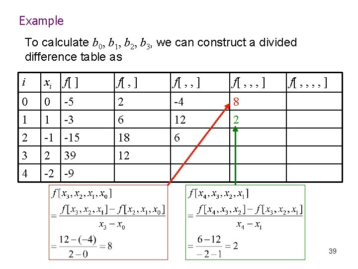
Example To calculate b 0, b 1, b 2, b 3, we can construct a divided difference table as i xi 0 1 2 3 4 f[ ] f[ , , ] 0 -5 1 -3 -1 -15 2 6 18 -4 12 6 2 39 -2 -9 12 f[ , , , ] f[ , , ] 38

Example To calculate b 0, b 1, b 2, b 3, we can construct a divided difference table as i xi 0 1 2 3 4 f[ ] f[ , , , ] 0 -5 1 -3 -1 -15 2 6 18 -4 12 6 8 2 2 39 -2 -9 12 f[ , , ] 39

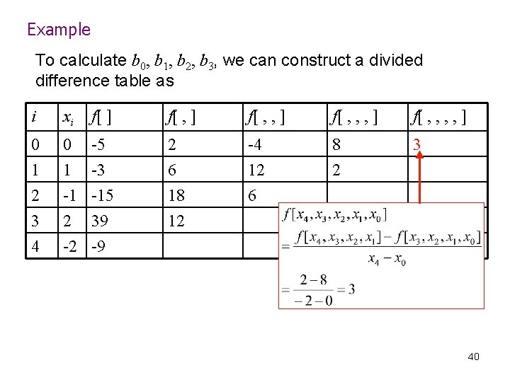
Example To calculate b 0, b 1, b 2, b 3, we can construct a divided difference table as i xi 0 1 2 3 4 f[ ] f[ , , , , ] 0 -5 1 -3 -1 -15 2 6 18 -4 12 6 8 2 39 -2 -9 12 40

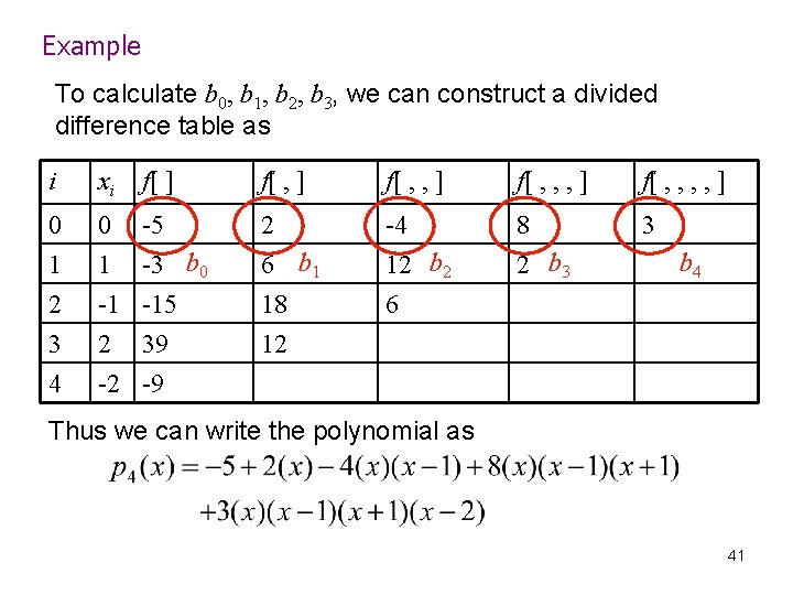
Example To calculate b 0, b 1, b 2, b 3, we can construct a divided difference table as i xi f[ ] f[ , , , , ] 0 1 2 0 -5 1 -3 b 0 -1 -15 2 6 b 1 18 -4 12 b 2 6 8 2 b 3 3 3 4 2 39 -2 -9 12 b 4 Thus we can write the polynomial as 41

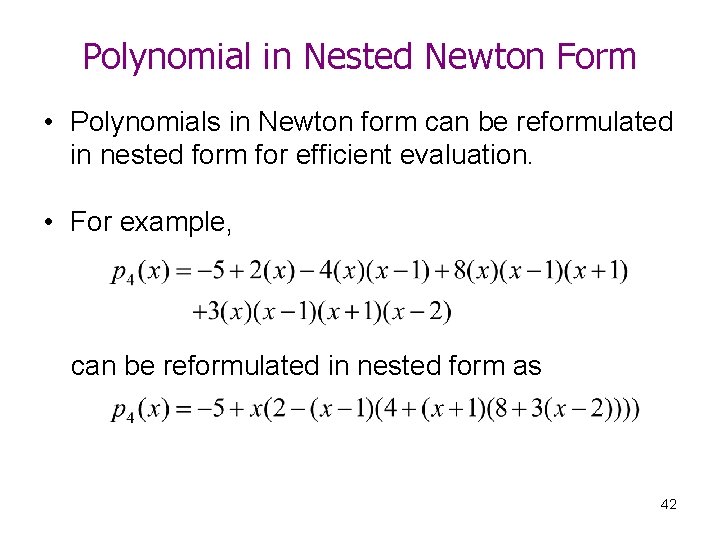
Polynomial in Nested Newton Form • Polynomials in Newton form can be reformulated in nested form for efficient evaluation. • For example, can be reformulated in nested form as 42

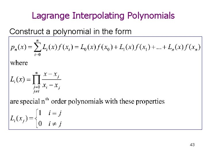
Lagrange Interpolating Polynomials Construct a polynomial in the form 43

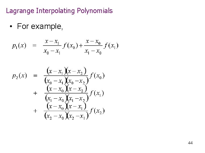
Lagrange Interpolating Polynomials • For example, 44

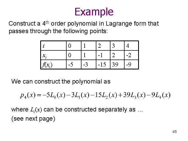
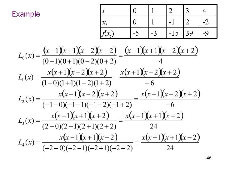
Example Construct a 4 th order polynomial in Lagrange form that passes through the following points: i xi f(xi) 0 0 -5 1 1 -3 2 3 -1 2 -15 39 4 -2 -9 We can construct the polynomial as where Li(x) can be constructed separately as … (see next page) 45

Example i xi f(xi) 0 0 -5 1 1 -3 2 3 -1 2 -15 39 4 -2 -9 46

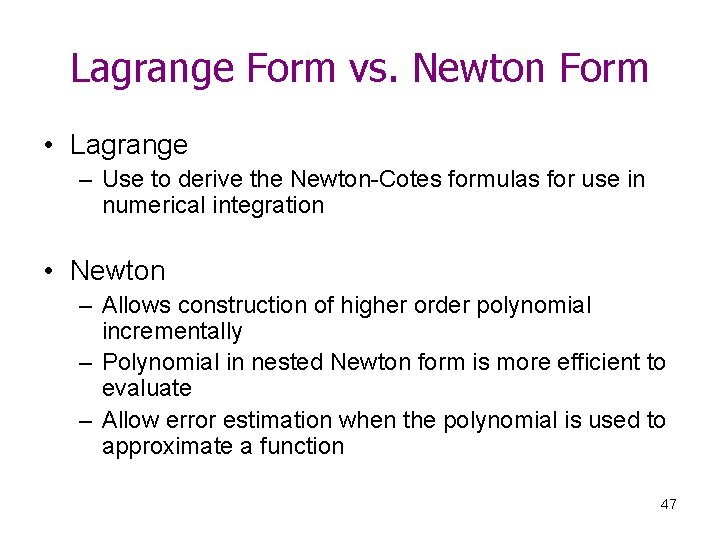
Lagrange Form vs. Newton Form • Lagrange – Use to derive the Newton-Cotes formulas for use in numerical integration • Newton – Allows construction of higher order polynomial incrementally – Polynomial in nested Newton form is more efficient to evaluate – Allow error estimation when the polynomial is used to approximate a function 47

Summary • Polynomial interpolation for approximate complicated functions. (Data are exact) • How to construct Newton and Lagrange Polynomial. – How to calculate divided difference of order n when given n+1 data points. 48

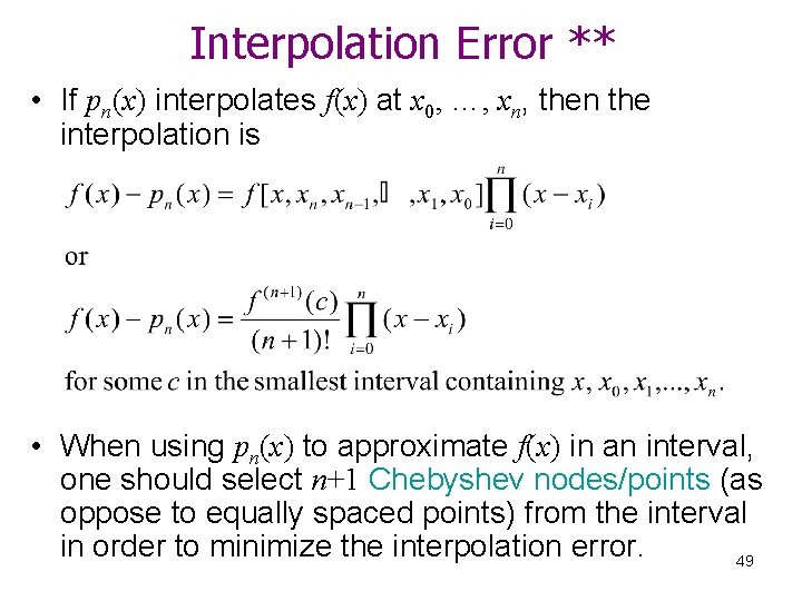
Interpolation Error ** • If pn(x) interpolates f(x) at x 0, …, xn, then the interpolation is • When using pn(x) to approximate f(x) in an interval, one should select n+1 Chebyshev nodes/points (as oppose to equally spaced points) from the interval in order to minimize the interpolation error. 49