Estimating Lp Norms Piotr Indyk MIT RecapToday Recap

Estimating Lp Norms Piotr Indyk MIT

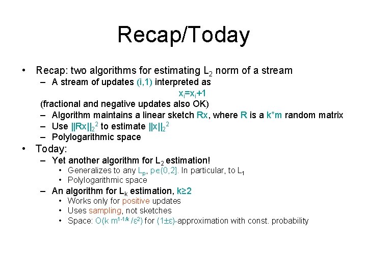
Recap/Today • Recap: two algorithms for estimating L 2 norm of a stream – A stream of updates (i, 1) interpreted as xi=xi+1 (fractional and negative updates also OK) – Algorithm maintains a linear sketch Rx, where R is a k*m random matrix – Use ||Rx||22 to estimate ||x||22 – Polylogarithmic space • Today: – Yet another algorithm for L 2 estimation! • Generalizes to any Lp, p (0, 2]. In particular, to L 1 • Polylogarithmic space – An algorithm for Lk estimation, k≥ 2 • Works only for positive updates • Uses sampling, not sketches • Space: O(k m 1 -1/k /ε 2) for (1 ε)-approximation with const. probability

L 2 estimation, version 3. 0

Median Estimator • • • Again we use a linear sketch Rx=[Z 1…Zk], where each entry of R has distribution N(0, 1), k=O(1/ε 2) – Therefore, each of Zi has N(0, 1) distribution with variance ∑i xi 2=||x||22 – Alternatively, Zi = ||x||2 Gi , where Gi drawn from N(0, 1) How to estimate ||x||2 from Z 1…Zk ? In Algorithms I, II, we used Y=[Z 12 + … +Zk 2]/k to estimate ||x||22 But there are many other estimators out there… E. g. , we could instead use Y=median*[ |Z 1|, … , |Zk| ]/ median**[|G|] • to estimate ||x||2 (G drawn from N(0, 1)) The rationale: – median [ |Z 1|, … , |Zk| ] = ||x||2 median [ |G 1|, … , |Gk | ] – For “large enough” k , median [ |G 1|, … , |Gk | ] is “close to” median[|G|] (next two slides) * median of an array A of numbers is the usual number in the middle of the sorted A ** M is the median of a random variable U if Pr[U≤M]=½

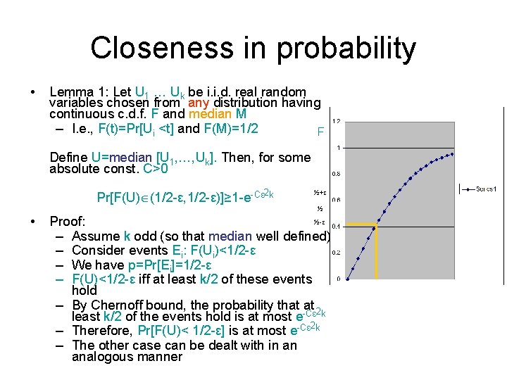
Closeness in probability • Lemma 1: Let U 1 … Uk be i. i. d. real random variables chosen from any distribution having continuous c. d. f. F and median M – I. e. , F(t)=Pr[Ui <t] and F(M)=1/2 F Define U=median [U 1, …, Uk]. Then, for some absolute const. C>0 Pr[F(U) (1/2 -ε, 1/2 -ε)]≥ 1 -e-Cε 2 k • ½+ε ½ ½-ε Proof: – Assume k odd (so that median well defined) – Consider events Ei: F(Ui)<1/2 -ε – We have p=Pr[Ei]=1/2 -ε – F(U)<1/2 -ε iff at least k/2 of these events hold – By Chernoff bound, the probability that at 2 least k/2 of the events hold is at most e-Cε k – Therefore, Pr[F(U)< 1/2 -ε] is at most e-Cε 2 k – The other case can be dealt with in an analogous manner

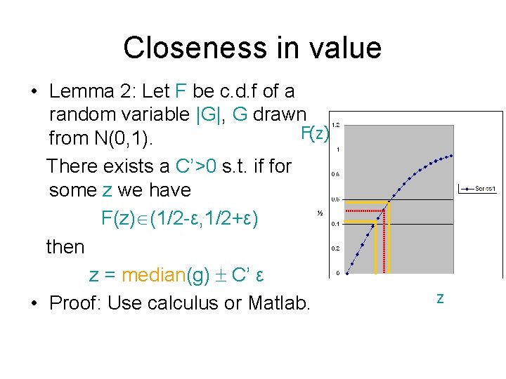
Closeness in value • Lemma 2: Let F be c. d. f of a random variable |G|, G drawn F(z) from N(0, 1). There exists a C’>0 s. t. if for some z we have F(z) (1/2 -ε, 1/2+ε) then z = median(g) C’ ε • Proof: Use calculus or Matlab. ½ z

Altogether • Theorem: If we use median estimator Y=median[ |Z 1|, … , |Zk|] / median[|g|] (where Zj=∑i rij xi , rij chosen i. i. d. from N(0, 1) ), then we have Y = ||x||2 [ median(g) C’ ε ] / median[|g|] = ||x||2 (1 C” ε) with probability 1 -e-Cε 2 k • How to extend this to ||x||p ?

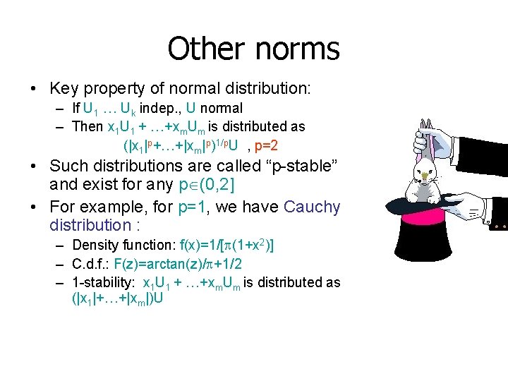
Other norms • Key property of normal distribution: – If U 1 … Uk indep. , U normal – Then x 1 U 1 + …+xm. Um is distributed as (|x 1|p+…+|xm|p)1/p. U , p=2 • Such distributions are called “p-stable” and exist for any p (0, 2] • For example, for p=1, we have Cauchy distribution : – Density function: f(x)=1/[ (1+x 2)] – C. d. f. : F(z)=arctan(z)/ +1/2 – 1 -stability: x 1 U 1 + …+xm. Um is distributed as (|x 1|+…+|xm|)U

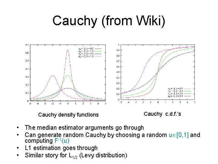
Cauchy (from Wiki) Cauchy density functions Cauchy c. d. f. ’s • The median estimator arguments go through • Can generate random Cauchy by choosing a random u [0, 1] and computing F-1(u) • L 1 estimation goes through • Similar story for L 1/2 (Levy distribution)

p-stability for p≠ 1, 2 , 1/2 • Basically, it is a mess – No closed formula for density/c. d. f. – Not clear where the median is – Not clear what the derivative of c. d. f. around the median is • Nevertheless – Can generate random variables – Moments are known (more or less) – Given samples of a*|g| , g p-stable, can estimate a up to 1 ε [Indyk, JACM’ 06; Ping Li, SODA’ 08] (using various hacks and/or moments) • For more info on p-stable distributions, see: V. V. Uchaikin, V. M. Zolotarev, Chance and Stability. Stable Distributions and their Applications. http: //staff. ulsu. ru/uchaikin/uchzol. pdf

Summary • Maintaining Lp norm of x under updates – Polylogarithmic space for p≤ 2 • Issues ignored: – Randomness – Discretization (but everything can be done using O(log (m+n)) bit numbers) • See [Kane-Nelson-Woodruff’ 10] on how to fix this (and get optimal bounds)

Lk norm, k≥ 2

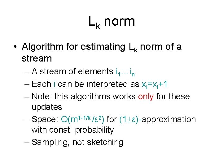
Lk norm • Algorithm for estimating Lk norm of a stream – A stream of elements i 1…in – Each i can be interpreted as xi=xi+1 – Note: this algorithms works only for these updates – Space: O(m 1 -1/k /ε 2) for (1 ε)-approximation with const. probability – Sampling, not sketching

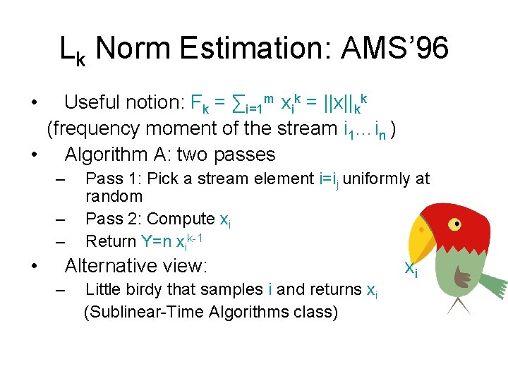
Lk Norm Estimation: AMS’ 96 • Useful notion: Fk = ∑i=1 m xik = ||x||kk (frequency moment of the stream i 1…in ) • Algorithm A: two passes – – – • Pass 1: Pick a stream element i=ij uniformly at random Pass 2: Compute xi Return Y=n xik-1 Alternative view: – Little birdy that samples i and returns xi (Sublinear-Time Algorithms class) xi

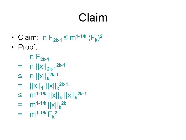
Analysis • Estimator Y=n xik-1 • Expectation E[Y]= ∑i xi/n * nxik-1 = ∑i xik =Fk • Second moment (≥variance) E[Y 2]= ∑i xi/n * n 2 xi 2 k-2 = n ∑i xi 2 k-1 = n F 2 k-1 • Claim (next slide): n F 2 k-1 ≤ m 1 -1/k (Fk)2 • Therefore, averaging over O(m 1 -1/k /ε 2) samples + Chebyshev does the job (Lecture 2)

Claim • Claim: n F 2 k-1 ≤ m 1 -1/k (Fk)2 • Proof: n F 2 k-1 = n ||x||2 k-1 ≤ n ||x||k 2 k-1 = ||x||1 ||x||k 2 k-1 ≤ m 1 -1/k ||x||k 2 k-1 = m 1 -1/k ||x||k 2 k = m 1 -1/k Fk 2

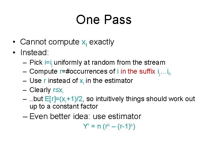
One Pass • Cannot compute xi exactly • Instead: – – – Pick i=ij uniformly at random from the stream Compute r=#occurrences of i in the suffix ij…in Use r instead of xi in the estimator Clearly r≤xi. . but E[r]=(xi+1)/2, so intuitively things should work out up to a constant factor – Even better idea: use estimator Y’ = n (rk – (r-1)k)

Analysis • Expectation: E[Y’] = n E[(rk – (r-1)k)] = n * 1/n ∑i ∑j=1 xi [jk – (j-1)k] = ∑i xik • Second moment: – Observe that Y’ = n (rk – (r-1)k) ≤ n k rk-1 ≤ k Y – Therefore E[Y’ 2 ] ≤ k 2 E[Y 2] ≤ k 2 m 1 -1/k Fk 2 (can improve to k m 1 -1/k Fk 2 for integer k) • Altogether, it proves: – One pass algorithm for Fk (positive updates) – Space: O(k 2 m 1 -1/k /ε 2) for (1 ε)-approximation

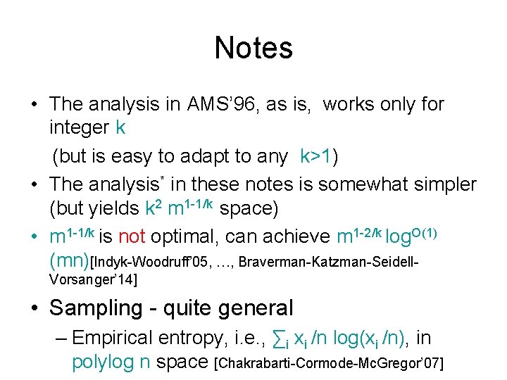
Notes • The analysis in AMS’ 96, as is, works only for integer k (but is easy to adapt to any k>1) • The analysis* in these notes is somewhat simpler (but yields k 2 m 1 -1/k space) • m 1 -1/k is not optimal, can achieve m 1 -2/k log. O(1) (mn)[Indyk-Woodruff’ 05, …, Braverman-Katzman-Seidell. Vorsanger’ 14] • Sampling - quite general – Empirical entropy, i. e. , ∑i xi /n log(xi /n), in polylog n space [Chakrabarti-Cormode-Mc. Gregor’ 07]