EE 313 Linear Systems and Signals Fall 2021

EE 313 Linear Systems and Signals Fall 2021 Continuous-Time Convolution Prof. Brian L. Evans Dept. of Electrical and Computer Engineering The University of Texas at Austin Textbook: Mc. Clellan, Schafer & Yoder, Signal Processing First, 2003 Lecture 13 http: //www. ece. utexas. edu/~bevans/courses/signals

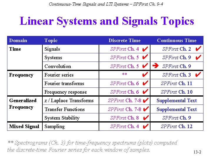
Continuous-Time Signals and LTI Systems – SPFirst Ch. 9 -4 Linear Systems and Signals Topics Domain Topic Discrete Time Signals SPFirst Ch. 2 ✔ ✔ SPFirst Ch. 5 ✔ SPFirst Ch. 9 ✔ SPFirst Ch. 5 ✔ SPFirst Ch. 9 ** SPFirst Ch. 3 ✔ ✔ SPFirst Ch. 6 ✔ SPFirst Ch. 11 SPFirst Ch. 6 ✔ SPFirst Ch. 10 SPFirst Ch. 7 -8 ✔ Supplemental Text SPFirst Ch. 8 ✔ SPFirst Ch. 9 SPFirst Ch. 4 ✔ SPFirst Ch. 12 Systems Convolution Frequency Fourier series Fourier transforms Frequency response Generalized Frequency z / Laplace Transforms Transfer Functions System Stability Mixed Signal Sampling Continuous Time SPFirst Ch. 4 ** Spectrograms (Ch. 3) for time-frequency spectrums (plots) computed the discrete-time Fourier series for each window of samples. 13 -2

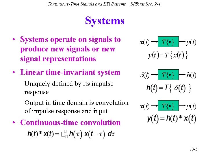
Continuous-Time Signals and LTI Systems – SPFirst Sec. 9 -4 Systems • Systems operate on signals to produce new signals or new signal representations • Linear time-invariant system x(t) T{ • } y(t) d(t) T{ • } h(t) x(t) T{ • } y(t) Uniquely defined by its impulse response Output in time domain is convolution of impulse response and input • Continuous-time convolution 13 -3

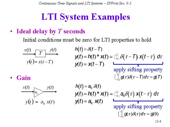
Continuous-Time Signals and LTI Systems – SPFirst Sec. 9 -5 LTI System Examples • Ideal delay by T seconds Initial conditions must be zero for LTI properties to hold x(t) y(t) apply sifting property • Gain x(t) y(t) apply sifting property 13 -4

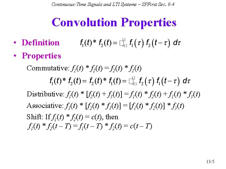
Continuous-Time Signals and LTI Systems – SPFirst Sec. 9 -4 Convolution Properties • Definition • Properties Commutative: f 1(t) * f 2(t) = f 2(t) * f 1(t) Distributive: f 1(t) * [f 2(t) + f 3(t)] = f 1(t) * f 2(t) + f 1(t) * f 3(t) Associative: f 1(t) * [f 2(t) * f 3(t)] = [f 1(t) * f 2(t)] * f 3(t) Shift: If f 1(t) * f 2(t) = c(t), then f 1(t) * f 2(t – T) = f 1(t – T) * f 2(t) = c(t – T) 13 -5

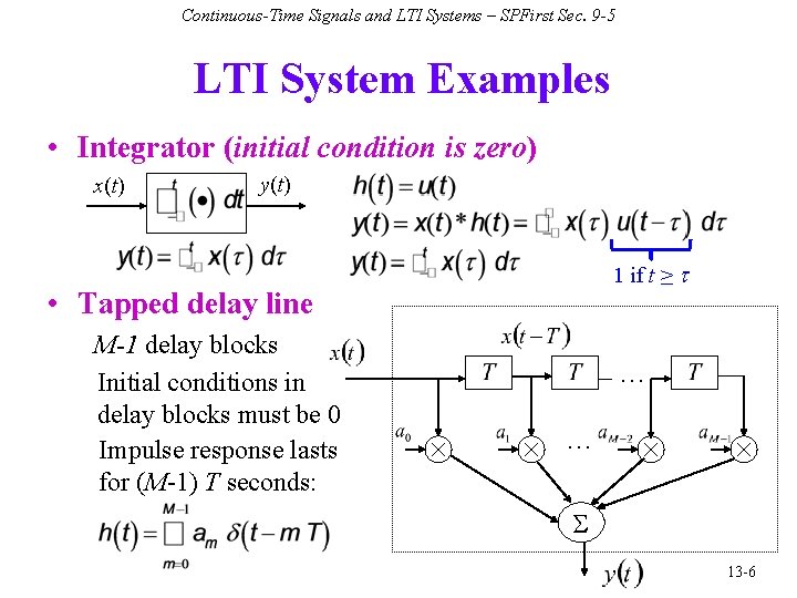
Continuous-Time Signals and LTI Systems – SPFirst Sec. 9 -5 LTI System Examples • Integrator (initial condition is zero) x(t) y(t) 1 if t ≥ t • Tapped delay line M-1 delay blocks Initial conditions in delay blocks must be 0 Impulse response lasts for (M-1) T seconds: … … S 13 -6

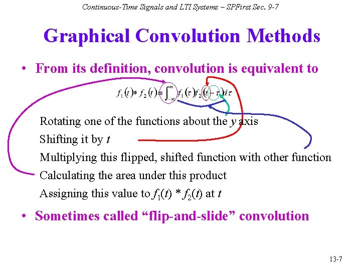
Continuous-Time Signals and LTI Systems – SPFirst Sec. 9 -7 Graphical Convolution Methods • From its definition, convolution is equivalent to Rotating one of the functions about the y axis Shifting it by t Multiplying this flipped, shifted function with other function Calculating the area under this product Assigning this value to f 1(t) * f 2(t) at t • Sometimes called “flip-and-slide” convolution 13 -7

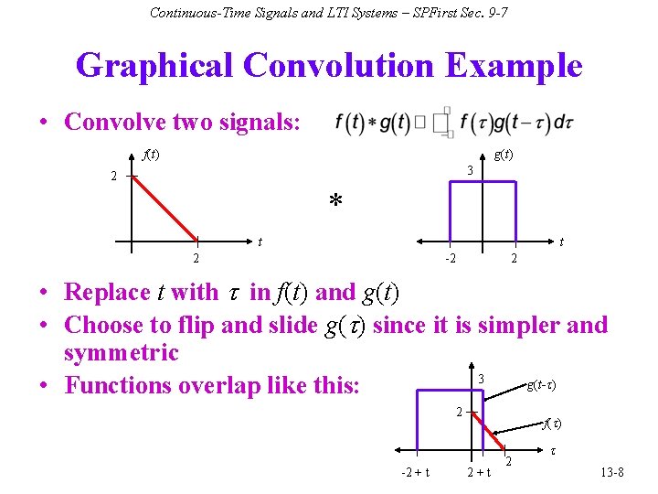
Continuous-Time Signals and LTI Systems – SPFirst Sec. 9 -7 Graphical Convolution Example • Convolve two signals: f(t) g(t) 3 2 * t t 2 -2 2 • Replace t with t in f(t) and g(t) • Choose to flip and slide g(t) since it is simpler and symmetric 3 g(t-t) • Functions overlap like this: 2 -2 + t f(t) 2+t 2 t 13 -8

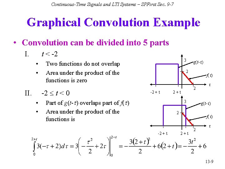
Continuous-Time Signals and LTI Systems – SPFirst Sec. 9 -7 Graphical Convolution Example • Convolution can be divided into 5 parts I. t < -2 • • -2 t < 0 II. • • 3 Two functions do not overlap Area under the product of the functions is zero g(t-t) 2 -2 + t Part of g(t-t) overlaps part of f(t) Area under the product of the functions is f(t) 2 2+t 3 g(t-t) 2 -2 + t t f(t) 2+t 2 t 13 -9

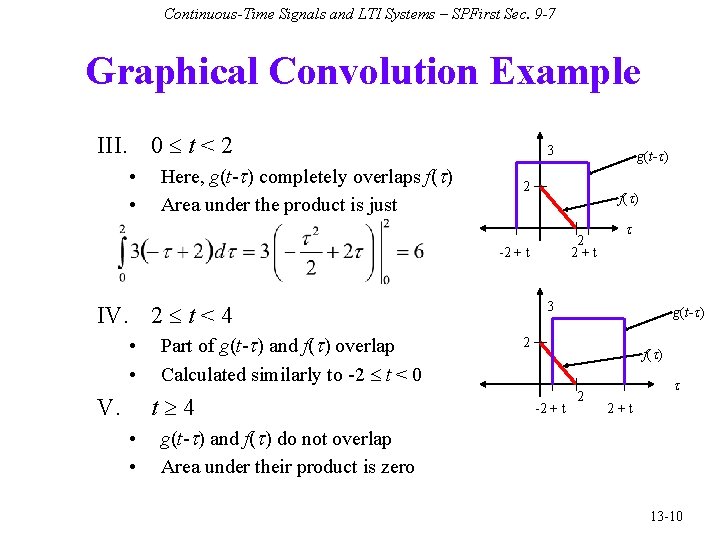
Continuous-Time Signals and LTI Systems – SPFirst Sec. 9 -7 Graphical Convolution Example III. 0 t < 2 • • Here, g(t-t) completely overlaps f(t) Area under the product is just 3 2 f(t) 2 2+t -2 + t IV. 2 t < 4 • • Part of g(t-t) and f(t) overlap Calculated similarly to -2 t < 0 t 4 V. • • g(t-t) t 3 g(t-t) 2 f(t) -2 + t 2+t g(t-t) and f(t) do not overlap Area under their product is zero 13 -10

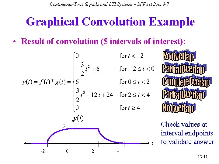
Continuous-Time Signals and LTI Systems – SPFirst Sec. 9 -7 Graphical Convolution Example • Result of convolution (5 intervals of interest): y(t) 6 t -2 0 2 Check values at interval endpoints to validate answer 4 13 -11

Continuous-Time Signals and LTI Systems – SPFirst Sec. 9 -7 Convolution Demos • Johns Hopkins University Demonstrations http: //pages. jh. edu/~signals/ Convolution applet to animate convolution of simple signals and hand-sketched signals Convolve two rectangular pulses of same width gives a triangle (see handout E) • Some conclusions from the animations Convolution of two causal signals gives a causal result Non-zero duration (called extent) of convolution is the sum of extents of the two signals being convolved 13 -12