EE 313 Linear Systems and Signals Fall 2021

EE 313 Linear Systems and Signals Fall 2021 Sampling Theorem Prof. Brian L. Evans Dept. of Electrical and Computer Engineering The University of Texas at Austin Textbook: Mc. Clellan, Schafer & Yoder, Signal Processing First, 2003 Lecture 6 http: //www. ece. utexas. edu/~bevans/courses/signals

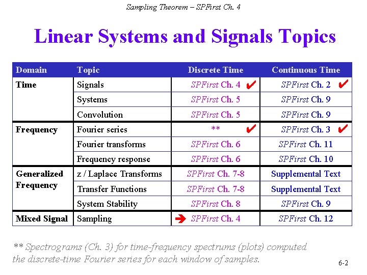
Sampling Theorem – SPFirst Ch. 4 Linear Systems and Signals Topics Domain Topic Discrete Time Signals SPFirst Ch. 4 Systems SPFirst Ch. 5 SPFirst Ch. 9 Convolution SPFirst Ch. 5 SPFirst Ch. 9 Fourier series ** Frequency Generalized Frequency ✔ ✔ SPFirst Ch. 2 SPFirst Ch. 3 ✔ ✔ Fourier transforms SPFirst Ch. 6 SPFirst Ch. 11 Frequency response SPFirst Ch. 6 SPFirst Ch. 10 z / Laplace Transforms SPFirst Ch. 7 -8 Supplemental Text Transfer Functions SPFirst Ch. 7 -8 Supplemental Text SPFirst Ch. 8 SPFirst Ch. 9 SPFirst Ch. 4 SPFirst Ch. 12 System Stability Mixed Signal Continuous Time Sampling ** Spectrograms (Ch. 3) for time-frequency spectrums (plots) computed the discrete-time Fourier series for each window of samples. 6 -2

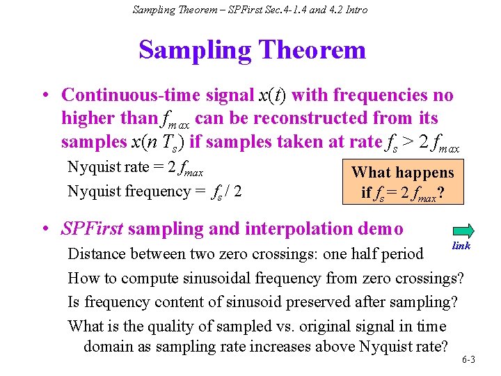
Sampling Theorem – SPFirst Sec. 4 -1. 4 and 4. 2 Intro Sampling Theorem • Continuous-time signal x(t) with frequencies no higher than fmax can be reconstructed from its samples x(n Ts) if samples taken at rate fs > 2 fmax Nyquist rate = 2 fmax Nyquist frequency = fs / 2 What happens if fs = 2 fmax? • SPFirst sampling and interpolation demo link Distance between two zero crossings: one half period How to compute sinusoidal frequency from zero crossings? Is frequency content of sinusoid preserved after sampling? What is the quality of sampled vs. original signal in time domain as sampling rate increases above Nyquist rate? 6 -3

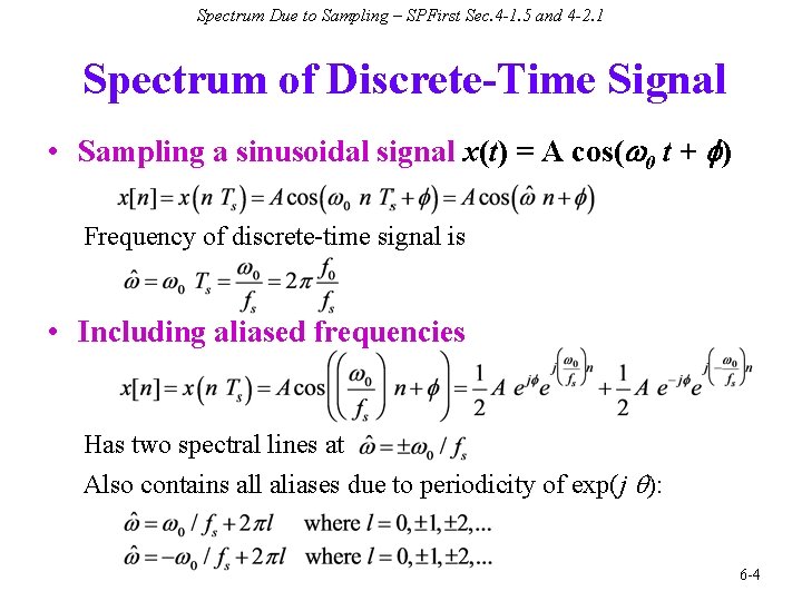
Spectrum Due to Sampling – SPFirst Sec. 4 -1. 5 and 4 -2. 1 Spectrum of Discrete-Time Signal • Sampling a sinusoidal signal x(t) = A cos(w 0 t + f) Frequency of discrete-time signal is • Including aliased frequencies Has two spectral lines at Also contains all aliases due to periodicity of exp(j q): 6 -4

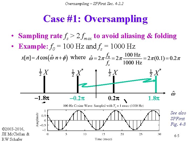
Oversampling – SPFirst Sec. 4 -2. 2 Case #1: Oversampling • Sampling rate fs > 2 fmax to avoid aliasing & folding • Example: f 0 = 100 Hz and fs = 1000 Hz where – 1. 8 p © 2003 -2016, JH Mc. Clellan & RW Schafer – 0. 2 p 1. 8 p See also SPFirst Fig. 4 -8 6 -5

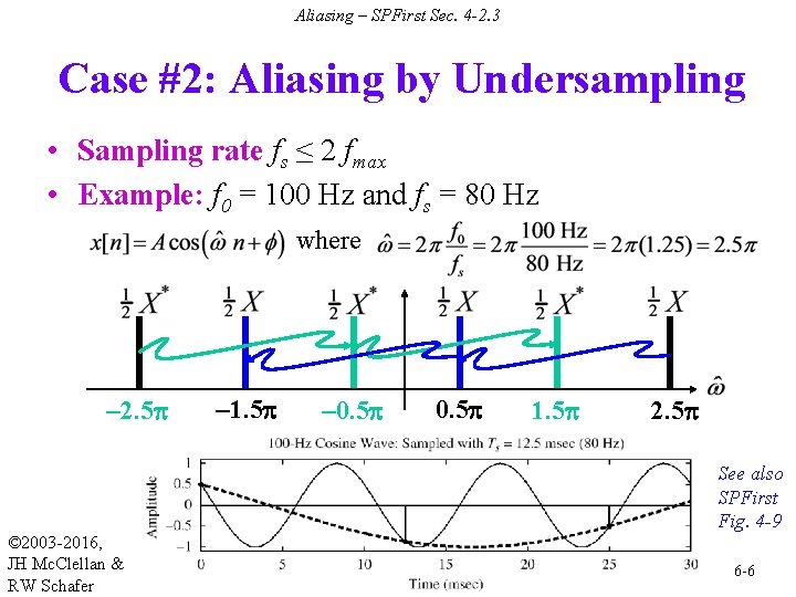
Aliasing – SPFirst Sec. 4 -2. 3 Case #2: Aliasing by Undersampling • Sampling rate fs ≤ 2 fmax • Example: f 0 = 100 Hz and fs = 80 Hz where – 2. 5 p – 1. 5 p – 0. 5 p 1. 5 p 2. 5 p See also SPFirst Fig. 4 -9 © 2003 -2016, JH Mc. Clellan & RW Schafer 6 -6

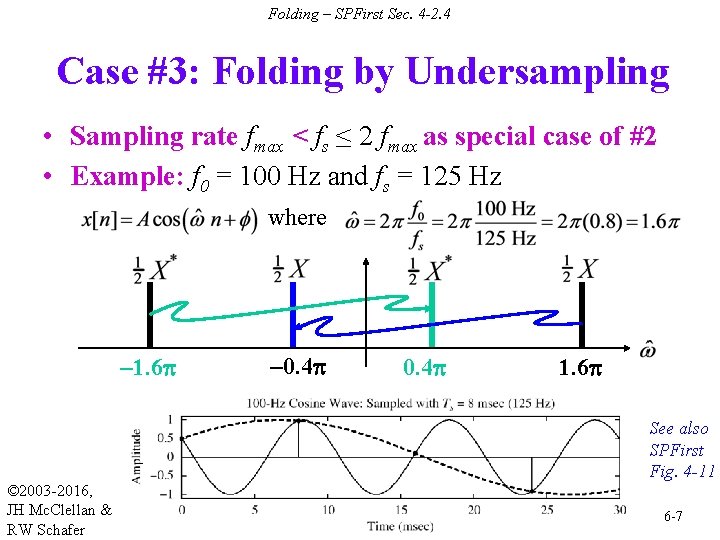
Folding – SPFirst Sec. 4 -2. 4 Case #3: Folding by Undersampling • Sampling rate fmax < fs ≤ 2 fmax as special case of #2 • Example: f 0 = 100 Hz and fs = 125 Hz where – 1. 6 p – 0. 4 p 1. 6 p See also SPFirst Fig. 4 -11 © 2003 -2016, JH Mc. Clellan & RW Schafer 6 -7

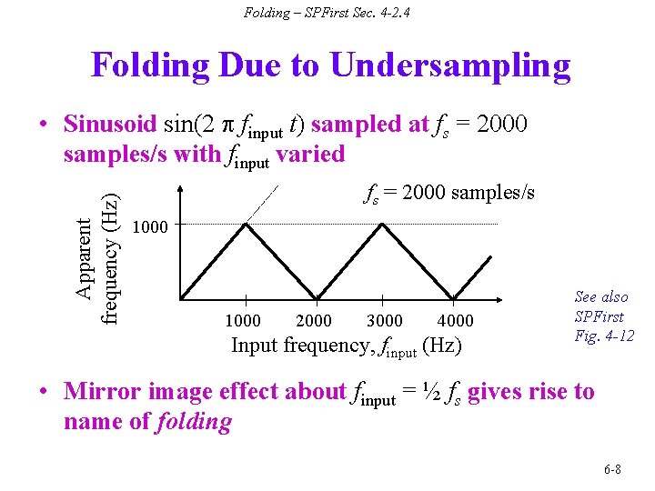
Folding – SPFirst Sec. 4 -2. 4 Folding Due to Undersampling Apparent frequency (Hz) • Sinusoid sin(2 finput t) sampled at fs = 2000 samples/s with finput varied fs = 2000 samples/s 1000 2000 3000 4000 Input frequency, finput (Hz) See also SPFirst Fig. 4 -12 • Mirror image effect about finput = ½ fs gives rise to name of folding 6 -8

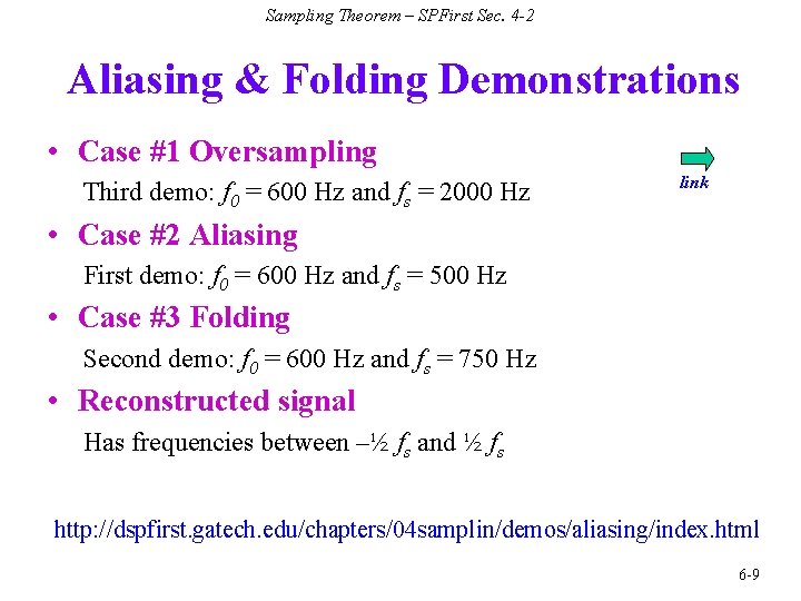
Sampling Theorem – SPFirst Sec. 4 -2 Aliasing & Folding Demonstrations • Case #1 Oversampling Third demo: f 0 = 600 Hz and fs = 2000 Hz link • Case #2 Aliasing First demo: f 0 = 600 Hz and fs = 500 Hz • Case #3 Folding Second demo: f 0 = 600 Hz and fs = 750 Hz • Reconstructed signal Has frequencies between –½ fs and ½ fs http: //dspfirst. gatech. edu/chapters/04 samplin/demos/aliasing/index. html 6 -9

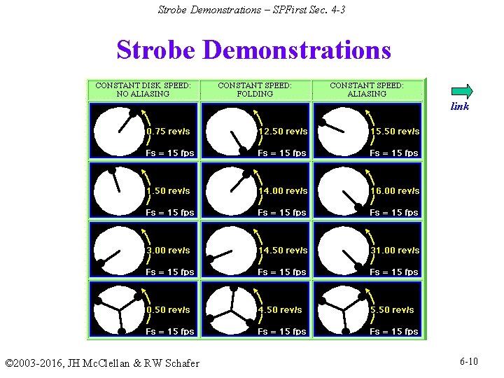
Strobe Demonstrations – SPFirst Sec. 4 -3 Strobe Demonstrations link © 2003 -2016, JH Mc. Clellan & RW Schafer 6 -10

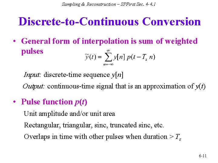
Sampling & Reconstruction – SPFirst Sec. 4 -4. 1 Discrete-to-Continuous Conversion • General form of interpolation is sum of weighted pulses Input: discrete-time sequence y[n] Output: continuous-time signal that is an approximation of y(t) • Pulse function p(t) Unit amplitude and/or unit area Rectangular, triangular, sinc, truncated sinc, etc. Overlaps in time with other pulses when duration > Ts 6 -11

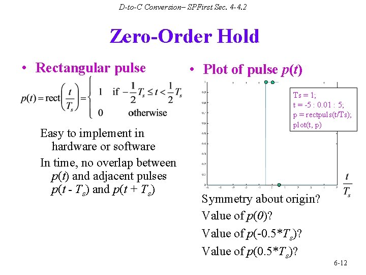
D-to-C Conversion– SPFirst Sec. 4 -4. 2 Zero-Order Hold • Rectangular pulse Easy to implement in hardware or software In time, no overlap between p(t) and adjacent pulses p(t - Ts) and p(t + Ts) • Plot of pulse p(t) Ts = 1; t = -5 : 0. 01 : 5; p = rectpuls(t/Ts); plot(t, p) Symmetry about origin? Value of p(0)? Value of p(-0. 5*Ts)? Value of p(0. 5*Ts)? 6 -12

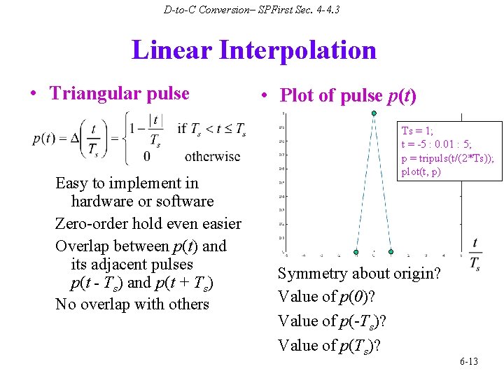
D-to-C Conversion– SPFirst Sec. 4 -4. 3 Linear Interpolation • Triangular pulse Easy to implement in hardware or software Zero-order hold even easier Overlap between p(t) and its adjacent pulses p(t - Ts) and p(t + Ts) No overlap with others • Plot of pulse p(t) Ts = 1; t = -5 : 0. 01 : 5; p = tripuls(t/(2*Ts)); plot(t, p) Symmetry about origin? Value of p(0)? Value of p(-Ts)? Value of p(Ts)? 6 -13

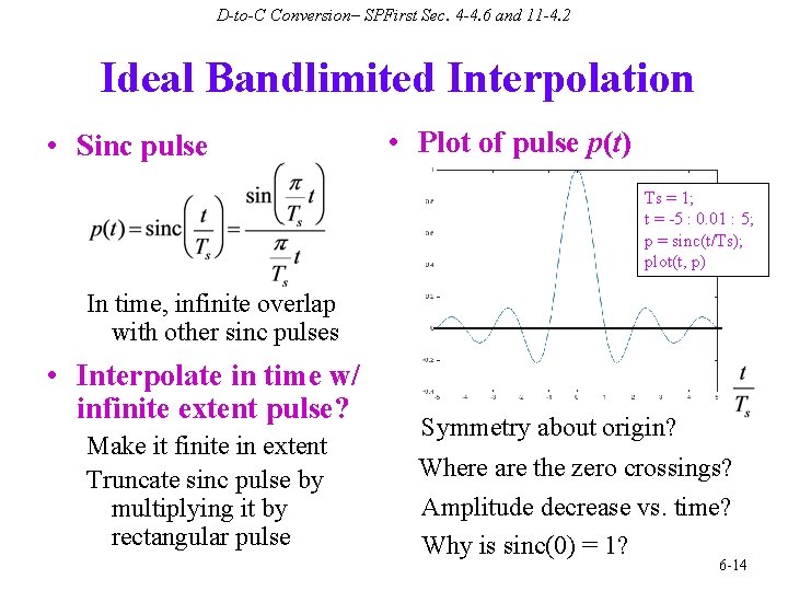
D-to-C Conversion– SPFirst Sec. 4 -4. 6 and 11 -4. 2 Ideal Bandlimited Interpolation • Sinc pulse • Plot of pulse p(t) Ts = 1; t = -5 : 0. 01 : 5; p = sinc(t/Ts); plot(t, p) In time, infinite overlap with other sinc pulses • Interpolate in time w/ infinite extent pulse? Make it finite in extent Truncate sinc pulse by multiplying it by rectangular pulse Symmetry about origin? Where are the zero crossings? Amplitude decrease vs. time? Why is sinc(0) = 1? 6 -14

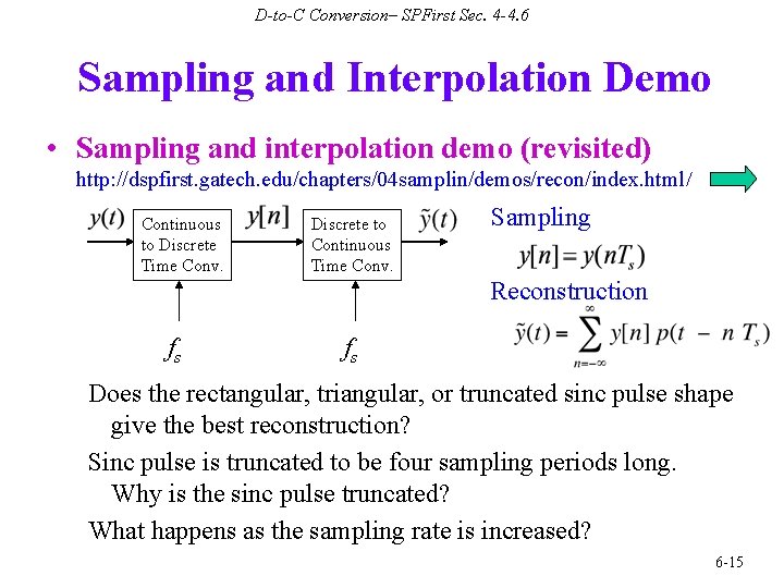
D-to-C Conversion– SPFirst Sec. 4 -4. 6 Sampling and Interpolation Demo • Sampling and interpolation demo (revisited) http: //dspfirst. gatech. edu/chapters/04 samplin/demos/recon/index. html/ Continuous to Discrete Time Conv. Discrete to Continuous Time Conv. Sampling Reconstruction fs fs Does the rectangular, triangular, or truncated sinc pulse shape give the best reconstruction? Sinc pulse is truncated to be four sampling periods long. Why is the sinc pulse truncated? What happens as the sampling rate is increased? 6 -15

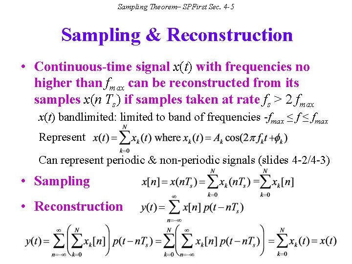
Sampling Theorem– SPFirst Sec. 4 -5 Sampling & Reconstruction • Continuous-time signal x(t) with frequencies no higher than fmax can be reconstructed from its samples x(n Ts) if samples taken at rate fs > 2 fmax x(t) bandlimited: limited to band of frequencies -fmax ≤ fmax Represent Can represent periodic & non-periodic signals (slides 4 -2/4 -3) • Sampling • Reconstruction