EE 313 Linear Systems and Signals Fall 2021

EE 313 Linear Systems and Signals Fall 2021 Sampling and Reconstruction Prof. Brian L. Evans Dept. of Electrical and Computer Engineering The University of Texas at Austin Textbook: Mc. Clellan, Schafer & Yoder, Signal Processing First, 2003 Lecture 16 http: //www. ece. utexas. edu/~bevans/courses/signals

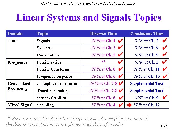
Continuous-Time Fourier Transform – SPFirst Ch. 12 Intro Linear Systems and Signals Topics Domain Topic Discrete Time Signals SPFirst Ch. 2 ✔ ✔ SPFirst Ch. 5 ✔ SPFirst Ch. 9 ✔ ** SPFirst Ch. 3 ✔ ✔ SPFirst Ch. 6 ✔ SPFirst Ch. 11 ✔ SPFirst Ch. 6 ✔ SPFirst Ch. 10 ✔ SPFirst Ch. 7 -8 ✔ Supplemental Text SPFirst Ch. 8 ✔ SPFirst Ch. 9 ✔ SPFirst Ch. 4 ✔ SPFirst Ch. 12 Systems Convolution Frequency Fourier series Fourier transforms Frequency response Generalized Frequency z / Laplace Transforms Transfer Functions System Stability Mixed Signal Sampling Continuous Time SPFirst Ch. 4 ** Spectrograms (Ch. 3) for time-frequency spectrums (plots) computed the discrete-time Fourier series for each window of samples. 16 -2

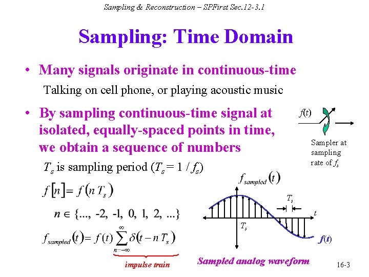
Sampling & Reconstruction – SPFirst Sec. 12 -3. 1 Sampling: Time Domain • Many signals originate in continuous-time Talking on cell phone, or playing acoustic music • By sampling continuous-time signal at isolated, equally-spaced points in time, we obtain a sequence of numbers f(t) Sampler at sampling rate of fs Ts is sampling period (Ts = 1 / fs) Ts t Ts f(t) impulse train Sampled analog waveform 16 -3

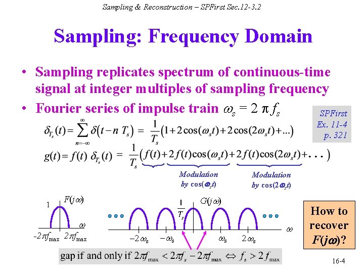
Sampling & Reconstruction – SPFirst Sec. 12 -3. 2 Sampling: Frequency Domain • Sampling replicates spectrum of continuous-time signal at integer multiples of sampling frequency • Fourier series of impulse train ws = 2 p fs SPFirst Ex. 11 -4 p. 321 Modulation by cos( st) 1 F(jw) Modulation by cos(2 st) G(jw) w -2 pfmax -2 ws - ws ws 2 ws w How to recover F(j )? 16 -4

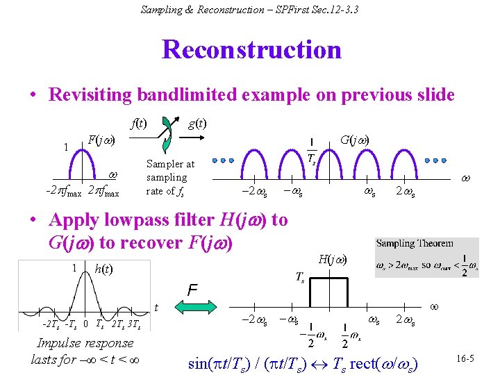
Sampling & Reconstruction – SPFirst Sec. 12 -3. 3 Reconstruction • Revisiting bandlimited example on previous slide f(t) g(t) G(jw) F(jw) 1 w -2 pfmax Sampler at sampling rate of fs -2 ws - ws • Apply lowpass filter H(j ) to G(j ) to recover F(j ) 1 h(t) ws 2 ws H(jw) F t -2 Ts -Ts 0 Ts 2 Ts 3 Ts Impulse response lasts for –∞ < t < ∞ -2 ws - ws w ws 2 ws sin(pt/Ts) / (pt/Ts) Ts rect(w/ws) w 16 -5

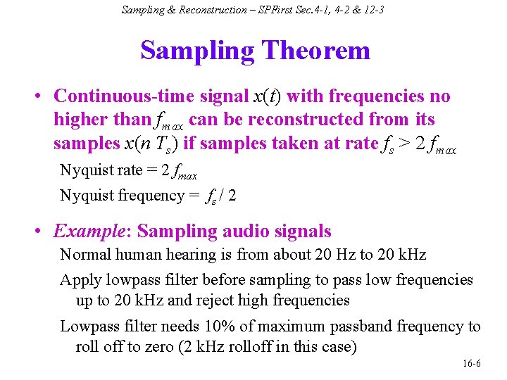
Sampling & Reconstruction – SPFirst Sec. 4 -1, 4 -2 & 12 -3 Sampling Theorem • Continuous-time signal x(t) with frequencies no higher than fmax can be reconstructed from its samples x(n Ts) if samples taken at rate fs > 2 fmax Nyquist rate = 2 fmax Nyquist frequency = fs / 2 • Example: Sampling audio signals Normal human hearing is from about 20 Hz to 20 k. Hz Apply lowpass filter before sampling to pass low frequencies up to 20 k. Hz and reject high frequencies Lowpass filter needs 10% of maximum passband frequency to roll off to zero (2 k. Hz rolloff in this case) 16 -6

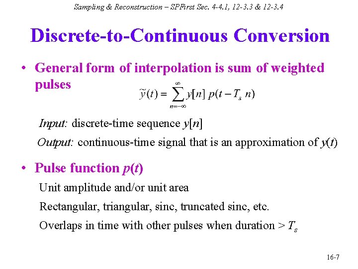
Sampling & Reconstruction – SPFirst Sec. 4 -4. 1, 12 -3. 3 & 12 -3. 4 Discrete-to-Continuous Conversion • General form of interpolation is sum of weighted pulses Input: discrete-time sequence y[n] Output: continuous-time signal that is an approximation of y(t) • Pulse function p(t) Unit amplitude and/or unit area Rectangular, triangular, sinc, truncated sinc, etc. Overlaps in time with other pulses when duration > Ts 16 -7

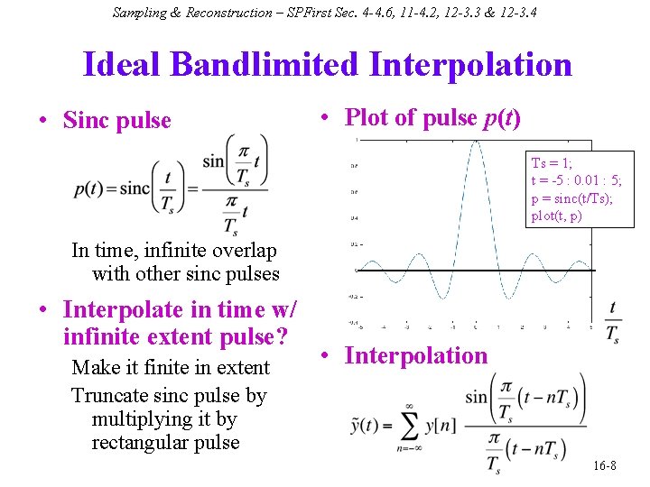
Sampling & Reconstruction – SPFirst Sec. 4 -4. 6, 11 -4. 2, 12 -3. 3 & 12 -3. 4 Ideal Bandlimited Interpolation • Sinc pulse • Plot of pulse p(t) Ts = 1; t = -5 : 0. 01 : 5; p = sinc(t/Ts); plot(t, p) In time, infinite overlap with other sinc pulses • Interpolate in time w/ infinite extent pulse? Make it finite in extent Truncate sinc pulse by multiplying it by rectangular pulse • Interpolation 16 -8