EE 313 Linear Systems and Signals Fall 2021

EE 313 Linear Systems and Signals Fall 2021 Z-Transforms Prof. Brian L. Evans Dept. of Electrical and Computer Engineering The University of Texas at Austin Textbook: Mc. Clellan, Schafer & Yoder, Signal Processing First, 2003 Lecture 10 http: //www. ece. utexas. edu/~bevans/courses/signals

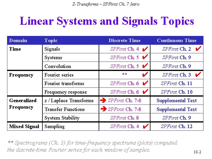
Z-Transforms – SPFirst Ch. 7 Intro Linear Systems and Signals Topics Domain Topic Discrete Time Signals SPFirst Ch. 4 Systems SPFirst Ch. 5 Convolution SPFirst Ch. 5 Fourier series ** Frequency Generalized Frequency Mixed Signal Fourier transforms SPFirst Ch. 6 Frequency response SPFirst Ch. 6 z / Laplace Transforms Transfer Functions Continuous Time ✔ ✔ ✔ SPFirst Ch. 7 -8 System Stability SPFirst Ch. 8 Sampling SPFirst Ch. 4 SPFirst Ch. 2 ✔ SPFirst Ch. 9 SPFirst Ch. 3 ✔ SPFirst Ch. 11 SPFirst Ch. 10 Supplemental Text SPFirst Ch. 9 ✔ SPFirst Ch. 12 ** Spectrograms (Ch. 3) for time-frequency spectrums (plots) computed the discrete-time Fourier series for each window of samples. 10 -2

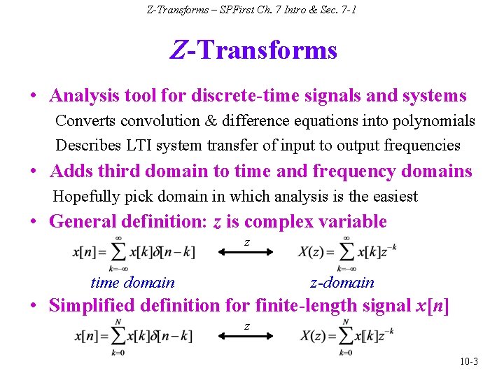
Z-Transforms – SPFirst Ch. 7 Intro & Sec. 7 -1 Z-Transforms • Analysis tool for discrete-time signals and systems Converts convolution & difference equations into polynomials Describes LTI system transfer of input to output frequencies • Adds third domain to time and frequency domains Hopefully pick domain in which analysis is the easiest • General definition: z is complex variable z time domain z-domain • Simplified definition for finite-length signal x[n] z 10 -3

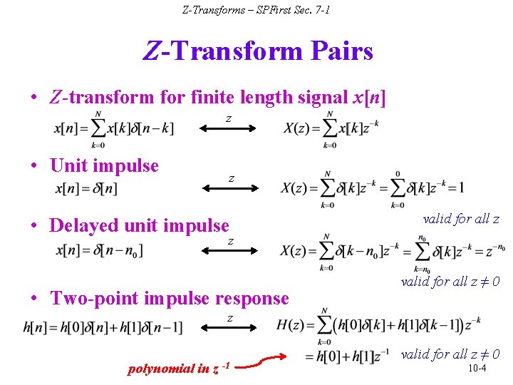
Z-Transforms – SPFirst Sec. 7 -1 Z-Transform Pairs • Z-transform for finite length signal x[n] z • Unit impulse z • Delayed unit impulse valid for all z z • Two-point impulse response valid for all z ≠ 0 z polynomial in z -1 valid for all z ≠ 0 10 -4

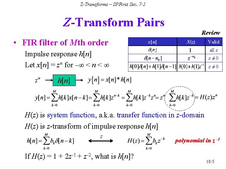
Z-Transforms – SPFirst Sec. 7 -2 Z-Transform Pairs Review • FIR filter of Mth order x[n] X(z) Valid all z Impulse response h[n] Let x[n] = zn for –∞ < n < ∞ z≠ 0 h[n] H(z) is system function, a. k. a. transfer function in z-domain H(z) is z-transform of impulse response h[n] z If H(z) = 1 + 2 z-1 + z-2, what is h[n]? polynomial in z -1 10 -5

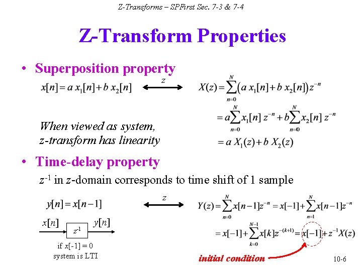
Z-Transforms – SPFirst Sec. 7 -3 & 7 -4 Z-Transform Properties • Superposition property z When viewed as system, z-transform has linearity • Time-delay property z-1 in z-domain corresponds to time shift of 1 sample z x[n] z-1 y[n] if x[-1] = 0 system is LTI initial condition 10 -6

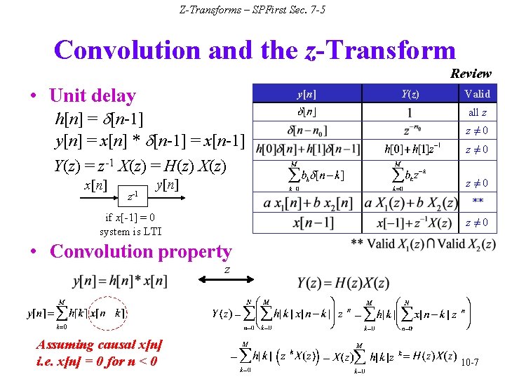
Z-Transforms – SPFirst Sec. 7 -5 Convolution and the z-Transform Review • Unit delay y[n] h[n] = d[n-1] y[n] = x[n] * d[n-1] = x[n-1] Y(z) = z-1 X(z) = H(z) X(z) x[n] z-1 y[n] Y(z) Valid all z z≠ 0 ** if x[-1] = 0 system is LTI z≠ 0 • Convolution property z Assuming causal x[n] i. e. x[n] = 0 for n < 0 10 -7

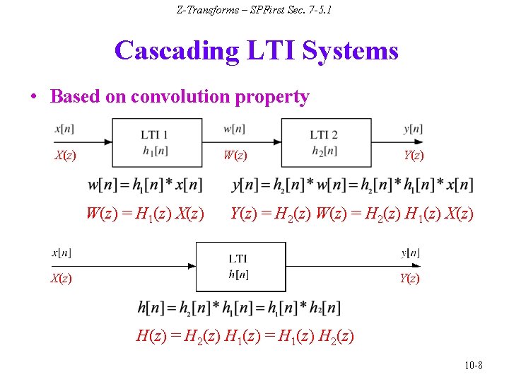
Z-Transforms – SPFirst Sec. 7 -5. 1 Cascading LTI Systems • Based on convolution property X(z) W(z) = H 1(z) X(z) Y(z) = H 2(z) W(z) = H 2(z) H 1(z) X(z) Y(z) H(z) = H 2(z) H 1(z) = H 1(z) H 2(z) 10 -8

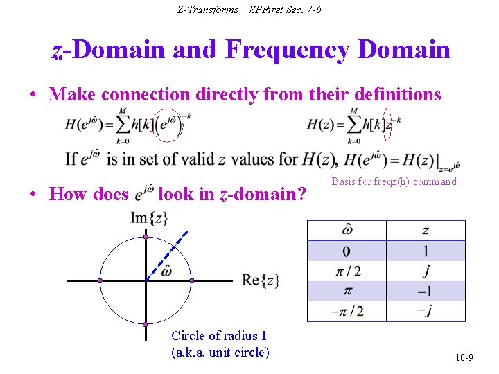
Z-Transforms – SPFirst Sec. 7 -6 z-Domain and Frequency Domain • Make connection directly from their definitions • How does look in z-domain? Circle of radius 1 (a. k. a. unit circle) Basis for freqz(h) command 10 -9

Z-Transforms – SPFirst Sec. 7 -6 & 7. 7 L-Point Averaging Filter h[n] • Impulse response: • Z-transform n -1 Roots of numerator (zeros): 0 1 2 L-1 L L=10 Roots of denominator (poles): Zero at z = 1 cancels pole at z = 1 h = (1/10)*ones(1, 10); zplane(h); 10 -10

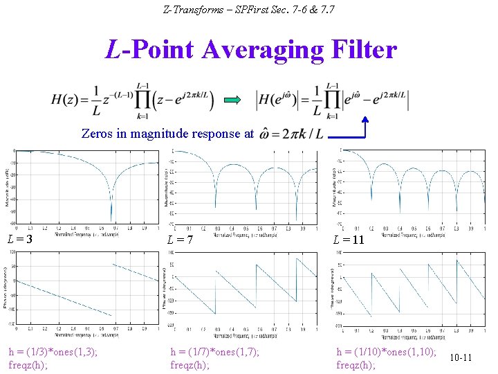
Z-Transforms – SPFirst Sec. 7 -6 & 7. 7 L-Point Averaging Filter Zeros in magnitude response at L=3 h = (1/3)*ones(1, 3); freqz(h); L=7 h = (1/7)*ones(1, 7); freqz(h); L = 11 h = (1/10)*ones(1, 10); freqz(h); 10 -11