Economics Review Antitrust Law Fall 2014 Yale Law

Economics Review Antitrust Law Fall 2014 Yale Law School Dale Collins

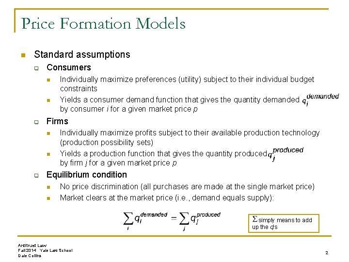
Price Formation Models n Standard assumptions q Consumers n n q Firms n n q Individually maximize preferences (utility) subject to their individual budget constraints Yields a consumer demand function that gives the quantity demanded by consumer i for a given market price p Individually maximize profits subject to their available production technology (production possibility sets) Yields a production function that gives the quantity produced by firm j for a given market price p Equilibrium condition n n No price discrimination (all purchases are made at the single market price) Market clears at the market price (i. e. , demand equals supply): simply means to add up the q’s Antitrust Law Fall 2014 Yale Law School Dale Collins 2

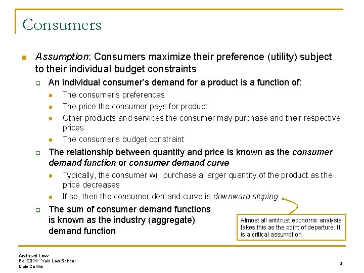
Consumers n Assumption: Consumers maximize their preference (utility) subject to their individual budget constraints q An individual consumer’s demand for a product is a function of: n n q The relationship between quantity and price is known as the consumer demand function or consumer demand curve n n q The consumer’s preferences The price the consumer pays for product Other products and services the consumer may purchase and their respective prices The consumer’s budget constraint Typically, the consumer will purchase a larger quantity of the product as the price decreases If so, then the consumer demand curve is downward sloping The sum of consumer demand functions is known as the industry (aggregate) demand function Antitrust Law Fall 2014 Yale Law School Dale Collins Almost all antitrust economic analysis takes this as the point of departure. It is a critical assumption. 3

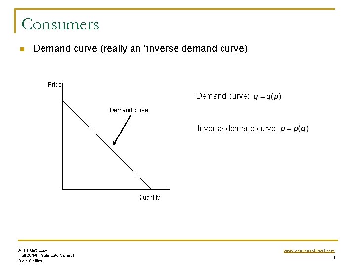
Consumers n Demand curve (really an “inverse demand curve) Price Demand curve: Demand curve Inverse demand curve: Quantity Antitrust Law Fall 2014 Yale Law School Dale Collins www. appliedantitrust. com 4

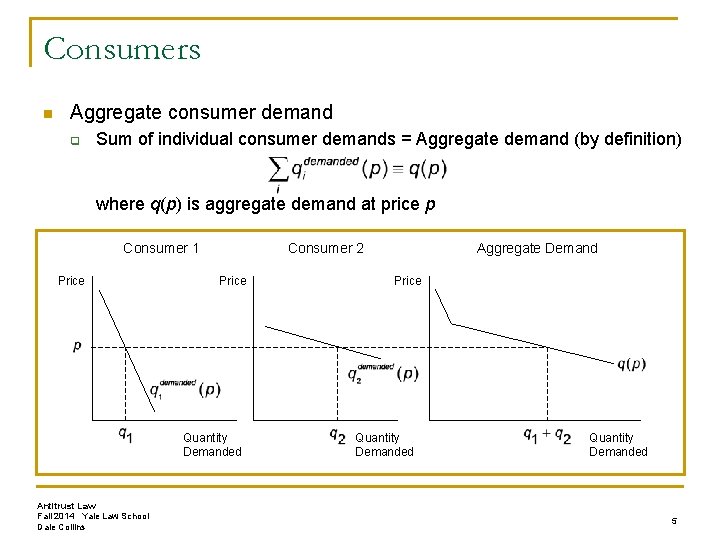
Consumers n Aggregate consumer demand q Sum of individual consumer demands = Aggregate demand (by definition) where q(p) is aggregate demand at price p Consumer 1 Price Consumer 2 Price Quantity Demanded Antitrust Law Fall 2014 Yale Law School Dale Collins Aggregate Demand Price Quantity Demanded 5

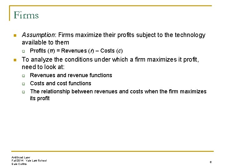
Firms n Assumption: Firms maximize their profits subject to the technology available to them q n Profits (π) = Revenues (r) – Costs (c) To analyze the conditions under which a firm maximizes it profit, need to look at: q q q Revenues and revenue functions Costs and cost functions The relationship between revenues and costs when the firm maximizes its profit Antitrust Law Fall 2014 Yale Law School Dale Collins 6

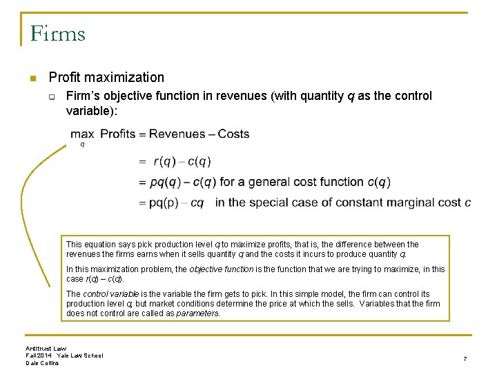
Firms n Profit maximization q Firm’s objective function in revenues (with quantity q as the control variable): This equation says pick production level q to maximize profits, that is, the difference between the revenues the firms earns when it sells quantity q and the costs it incurs to produce quantity q. In this maximization problem, the objective function is the function that we are trying to maximize, in this case r(q) ‒ c(q). The control variable is the variable the firm gets to pick. In this simple model, the firm can control its production level q, but market conditions determine the price at which the sells. Variables that the firm does not control are called as parameters. Antitrust Law Fall 2014 Yale Law School Dale Collins 7

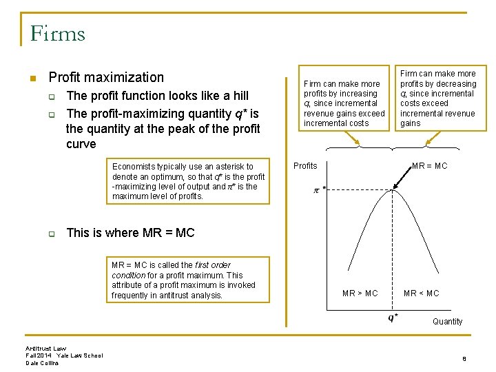
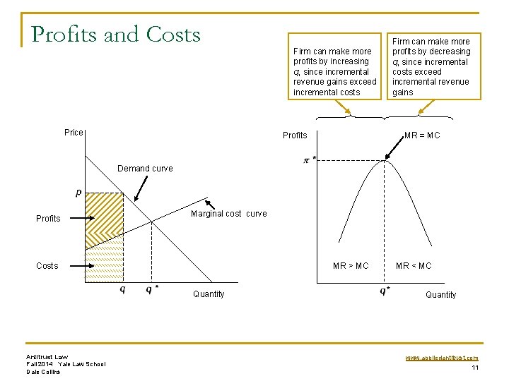
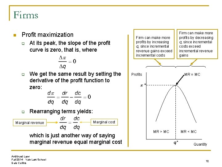
Firms n Profit maximization q q The profit function looks like a hill The profit-maximizing quantity q* is the quantity at the peak of the profit curve Economists typically use an asterisk to denote an optimum, so that q* is the profit -maximizing level of output and π* is the maximum level of profits. q Firm can make more profits by increasing q, since incremental revenue gains exceed incremental costs Firm can make more profits by decreasing q, since incremental costs exceed incremental revenue gains MR = MC Profits This is where MR = MC is called the first order condition for a profit maximum. This attribute of a profit maximum is invoked frequently in antitrust analysis. MR > MC MR < MC Quantity Antitrust Law Fall 2014 Yale Law School Dale Collins 8

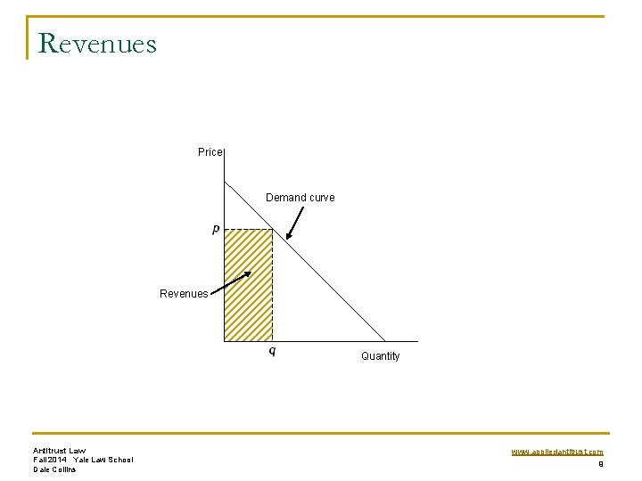
Revenues Price Demand curve Revenues Quantity Antitrust Law Fall 2014 Yale Law School Dale Collins www. appliedantitrust. com 9

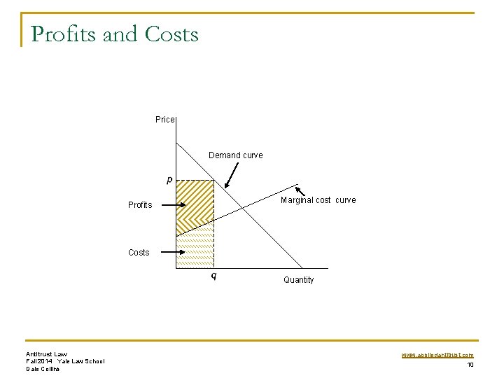
Profits and Costs Price Demand curve Profits Marginal cost curve Costs Quantity Antitrust Law Fall 2014 Yale Law School Dale Collins www. appliedantitrust. com 10

Profits and Costs Price Firm can make more profits by increasing q, since incremental revenue gains exceed incremental costs Firm can make more profits by decreasing q, since incremental costs exceed incremental revenue gains MR = MC Profits Demand curve Profits Marginal cost curve MR > MC Costs Quantity Antitrust Law Fall 2014 Yale Law School Dale Collins MR < MC Quantity www. appliedantitrust. com 11

Firms n Profit maximization q q q At its peak, the slope of the profit curve is zero, that is, where We get the same result by setting the derivative of the profit function to zero: Firm can make more profits by increasing q, since incremental revenue gains exceed incremental costs Firm can make more profits by decreasing q, since incremental costs exceed incremental revenue gains MR = MC Profits Rearranging terms yields: Marginal revenue Marginal cost which is just another way of saying marginal revenue equal marginal cost Antitrust Law Fall 2014 Yale Law School Dale Collins MR > MC MR < MC Quantity 12

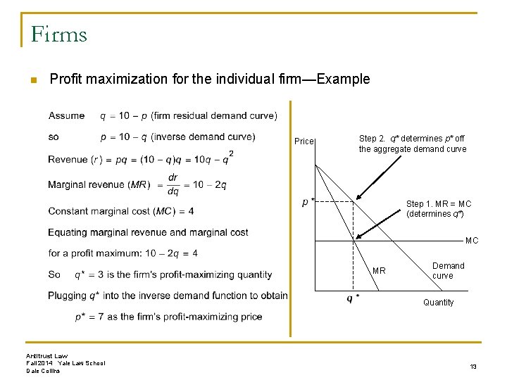
Firms n Profit maximization for the individual firm—Example Price Step 2. q* determines p* off the aggregate demand curve Step 1. MR = MC (determines q*) MC MR Demand curve Quantity Antitrust Law Fall 2014 Yale Law School Dale Collins 13

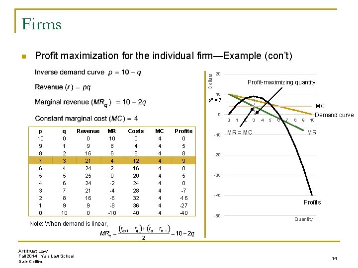
Firms Profit maximization for the individual firm—Example (con’t) Dollars n 20 Profit-maximizing quantity 10 p* = 7 0 0 p 10 9 8 7 6 5 4 3 2 1 0 q 0 1 2 3 4 5 6 7 8 9 10 Revenue 0 9 16 21 24 25 24 21 16 9 0 Note: When demand is linear, Antitrust Law Fall 2014 Yale Law School Dale Collins MR 10 8 6 4 2 0 -2 -4 -6 -8 -10 Costs 0 4 8 12 16 20 24 28 32 36 40 MC 4 4 4 Profits 0 5 8 9 8 5 0 -7 -16 -27 -40 -10 1 2 3 MR = MC 4 5 6 7 8 9 10 MC Demand curve MR -20 -30 -40 Profits -50 Quantity 14

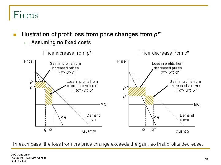
Firms n Illustration of profit loss from price changes from p* q Assuming no fixed costs Price increase from p* Price decrease from p* Price Gain in profits from increased prices = (p´- p*) q´ Loss in profits from decreased prices = (p* - p´´) q* Loss in profits from decreased volume = (q* - q´) p* Gain in profits from increased volume = (q* - q´´) p´´ MC MR Demand curve Quantity In each case, the loss from the price change exceeds the gain, so that profits decrease. Antitrust Law Fall 2014 Yale Law School Dale Collins 15

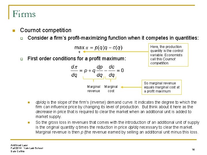
Firms n Cournot competition q q Consider a firm’s profit-maximizing function when it competes in quantities: First order conditions for a profit maximum: Marginal revenue n n Marginal cost Here, the production quantity is the control variable. Economists call this Cournot competition. So marginal revenue equals marginal cost at a profit maximum dp/dq is the slope of the firm’s (inverse) demand curve. It indicates the degree to which the firm can influence price by changing its level of production. But think about it here as the decrease in price that is required to clear the market when an additional unit is added to market supply. So the gross loss in revenues that comes with the introduction of an additional unit of supply is the original quantity q times the reduction in price dp/dq necessary to clear the market. Marginal revenue is then p (the revenue earned by selling an additional unit minus this loss. Antitrust Law Fall 2014 Yale Law School Dale Collins 16

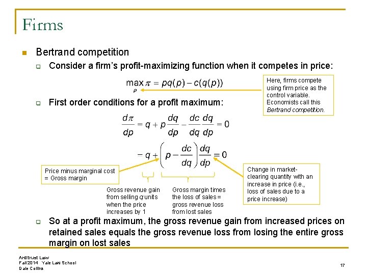
Firms n Bertrand competition q q Consider a firm’s profit-maximizing function when it competes in price: First order conditions for a profit maximum: Price minus marginal cost = Gross margin Gross revenue gain from selling q units when the price increases by 1 q Gross margin times the loss of sales = gross revenue loss from lost sales Here, firms compete using firm price as the control variable. Economists call this Bertrand competition. Change in marketclearing quantity with an increase in price (i. e. , loss of sales due to a price increase) So at a profit maximum, the gross revenue gain from increased prices on retained sales equals the gross revenue loss from losing the entire gross margin on lost sales Antitrust Law Fall 2014 Yale Law School Dale Collins 17

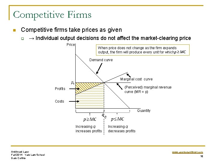
Competitive Firms n Competitive firms take prices as given q → Individual output decisions do not affect the market-clearing price Price When price does not change as the firm expands output, the firm will produce every unit for which Demand curve Marginal cost curve (Perceived) marginal revenue curve (MR = p) Profits Costs Quantity Increasing q increases profits Antitrust Law Fall 2014 Yale Law School Dale Collins Increasing q decreases profits www. appliedantitrust. com 18

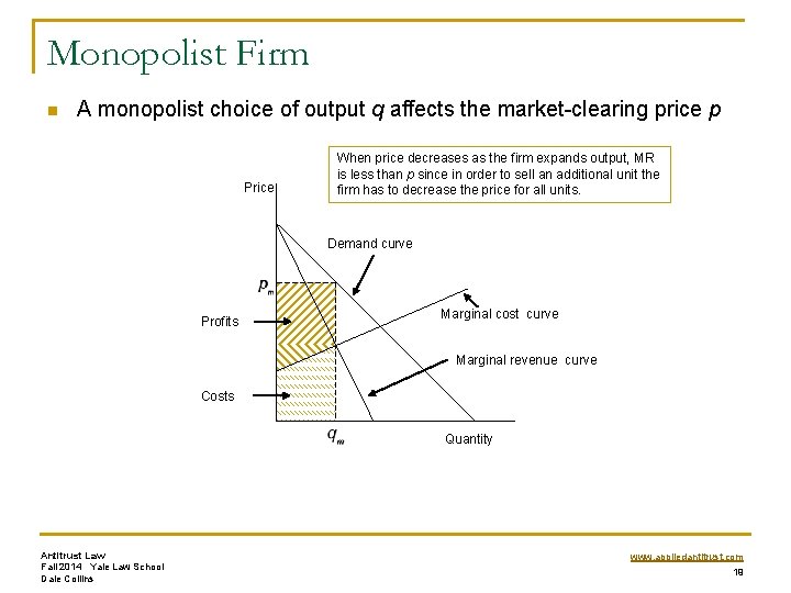
Monopolist Firm n A monopolist choice of output q affects the market-clearing price p Price When price decreases as the firm expands output, MR is less than p since in order to sell an additional unit the firm has to decrease the price for all units. Demand curve Profits Marginal cost curve Marginal revenue curve Costs Quantity Antitrust Law Fall 2014 Yale Law School Dale Collins www. appliedantitrust. com 19

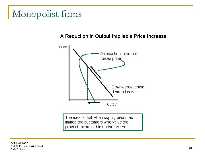
Monopolist firms A Reduction in Output Implies a Price Increase Price A reduction in output raises price Downward-sloping demand curve Output The idea is that when supply becomes limited the customers who value the product the most bid up the prices Antitrust Law Fall 2014 Yale Law School Dale Collins 20 §

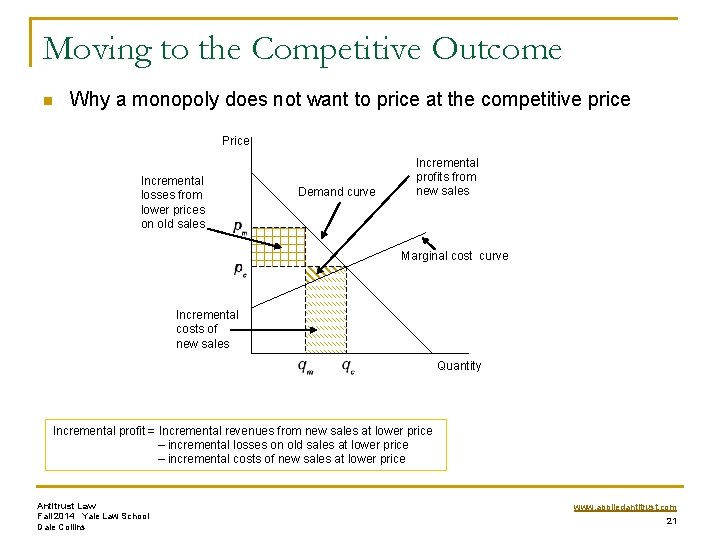
Moving to the Competitive Outcome n Why a monopoly does not want to price at the competitive price Price Incremental losses from lower prices on old sales Demand curve Incremental profits from new sales Marginal cost curve Incremental costs of new sales Quantity Incremental profit = Incremental revenues from new sales at lower price – incremental losses on old sales at lower price – incremental costs of new sales at lower price Antitrust Law Fall 2014 Yale Law School Dale Collins www. appliedantitrust. com 21

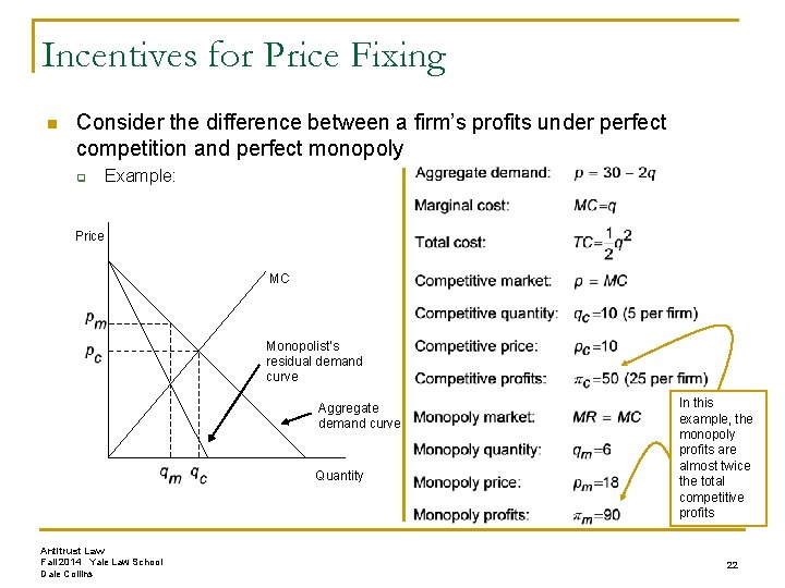
Incentives for Price Fixing n Consider the difference between a firm’s profits under perfect competition and perfect monopoly q Example: Price MC Monopolist’s residual demand curve Aggregate demand curve Quantity Antitrust Law Fall 2014 Yale Law School Dale Collins In this example, the monopoly profits are almost twice the total competitive profits 22

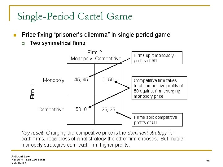
Single-Period Cartel Game n Price fixing “prisoner’s dilemma” in single period game q Two symmetrical firms Firm 2 Monopoly Competitive 45, 45 0, 50 Competitive 50, 0 25, 25 Firm 1 Monopoly Firms split monopoly profits of 90 Competitive firm takes total competitive profits of 50 against firm charging monopoly price Firms split competitive profits of 50 Key result: Charging the competitive price is the dominant strategy for each firms, regardless of what strategy the other firm chooses. But mutual monopoly strategies earn each firm higher profits. Antitrust Law Fall 2014 Yale Law School Dale Collins 23

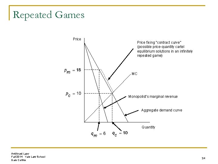
Repeated Games Price fixing “contract curve” (possible price-quantity cartel equilibrium solutions in an infinitely repeated game) MC Monopolist’s marginal revenue Aggregate demand curve Quantity Antitrust Law Fall 2014 Yale Law School Dale Collins 24

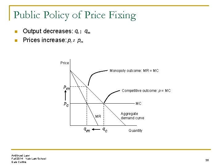
Public Policy of Price Fixing n n Output decreases: Prices increase: Price Monopoly outcome: MR = MC Competitive outcome: p = MC MC MR Aggregate demand curve Quantity Antitrust Law Fall 2014 Yale Law School Dale Collins 25

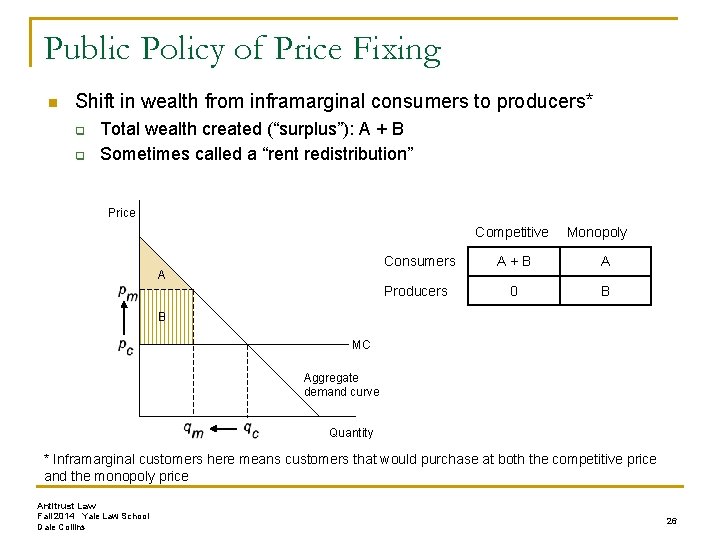
Public Policy of Price Fixing n Shift in wealth from inframarginal consumers to producers* q q Total wealth created (“surplus”): A + B Sometimes called a “rent redistribution” Price Competitive A Monopoly Consumers A+B A Producers 0 B B MC Aggregate demand curve Quantity * Inframarginal customers here means customers that would purchase at both the competitive price and the monopoly price Antitrust Law Fall 2014 Yale Law School Dale Collins 26

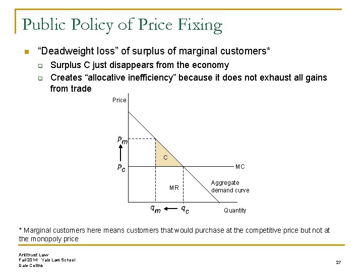
Public Policy of Price Fixing n “Deadweight loss” of surplus of marginal customers* q q Surplus C just disappears from the economy Creates “allocative inefficiency” because it does not exhaust all gains from trade Price C MC MR Aggregate demand curve Quantity * Marginal customers here means customers that would purchase at the competitive price but not at the monopoly price Antitrust Law Fall 2014 Yale Law School Dale Collins 27

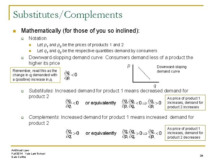
Substitutes/Complements n Mathematically (for those of you so inclined): q Notation n n q Let p 1 and p 2 be the prices of products 1 and 2 Let q 1 and q 2 be the respective quantities demand by consumers Downward-slopping demand curve: Consumers demand less of a product the higher its price p Downward-sloping Remember, read this as the change in qi demanded with a (positive) increase in pi q demand curve q Substitutes: Increased demand for product 1 means decreased demand for product 2 As price of product 1 increases, demand for product 2 increases q Complements: Increased demand for product 1 means increased demand for product 2 As price of product 1 increases, demand for product 2 decreases Antitrust Law Fall 2014 Yale Law School Dale Collins 28

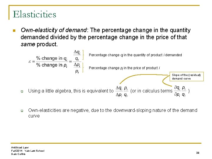
Elasticities n Own-elasticity of demand: The percentage change in the quantity demanded divided by the percentage change in the price of that same product. Percentage change qi in the quantity of product i demanded Percentage change pi in the price of product i Slope of the (residual) demand curve q q Using a little algebra, this is equivalent to (or in calculus terms ) Own-elasticities are negative, due to the downward-sloping nature of the demand curve Antitrust Law Fall 2014 Yale Law School Dale Collins 29

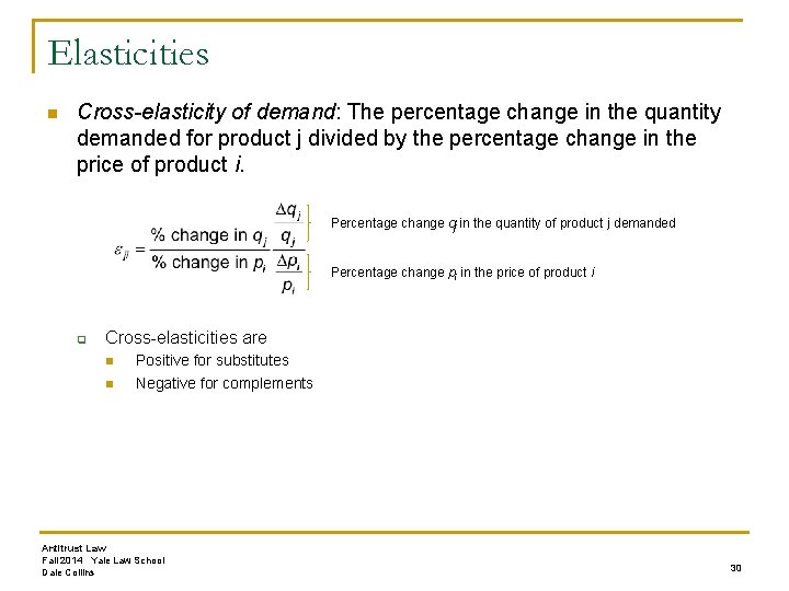
Elasticities n Cross-elasticity of demand: The percentage change in the quantity demanded for product j divided by the percentage change in the price of product i. Percentage change qj in the quantity of product j demanded Percentage change pi in the price of product i q Cross-elasticities are n n Positive for substitutes Negative for complements Antitrust Law Fall 2014 Yale Law School Dale Collins 30

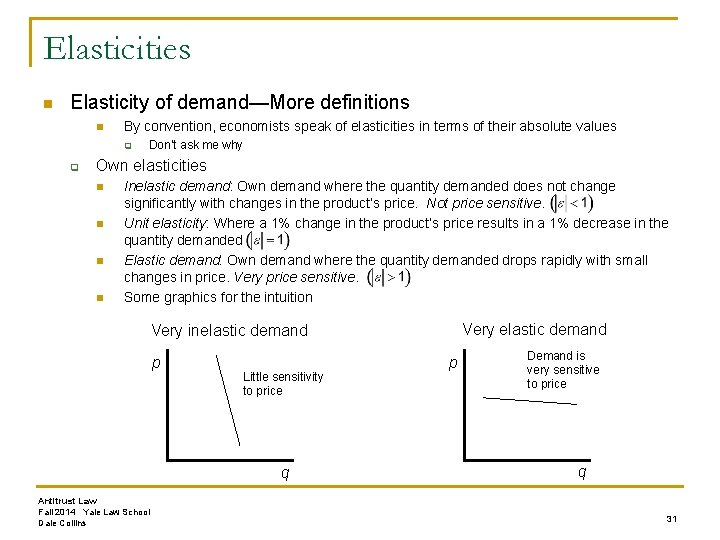
Elasticities n Elasticity of demand—More definitions n By convention, economists speak of elasticities in terms of their absolute values q q Don’t ask me why Own elasticities n n Inelastic demand: Own demand where the quantity demanded does not change significantly with changes in the product’s price. Not price sensitive. Unit elasticity: Where a 1% change in the product’s price results in a 1% decrease in the quantity demanded Elastic demand: Own demand where the quantity demanded drops rapidly with small changes in price. Very price sensitive. Some graphics for the intuition Very elastic demand Very inelastic demand p Little sensitivity to price q Antitrust Law Fall 2014 Yale Law School Dale Collins p Demand is very sensitive to price q 31

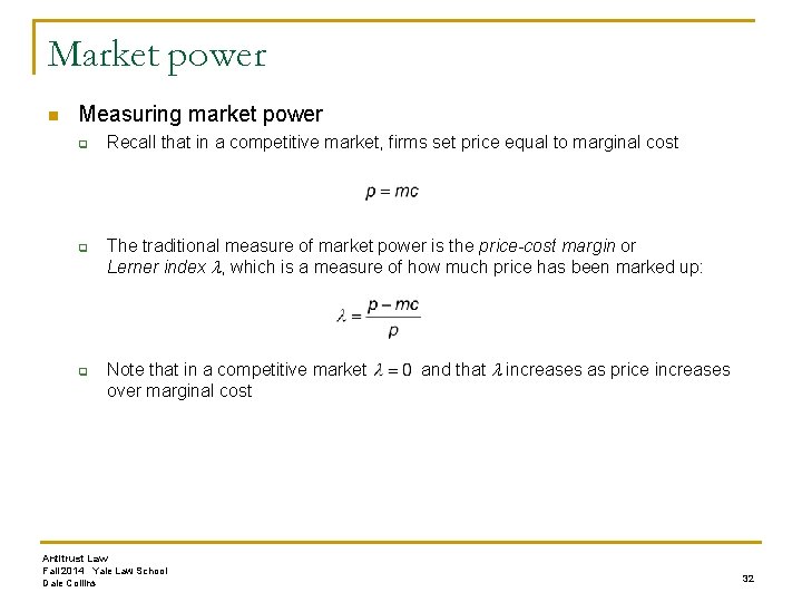
Market power n Measuring market power q q q Recall that in a competitive market, firms set price equal to marginal cost The traditional measure of market power is the price-cost margin or Lerner index , which is a measure of how much price has been marked up: Note that in a competitive market over marginal cost Antitrust Law Fall 2014 Yale Law School Dale Collins and that increases as price increases 32

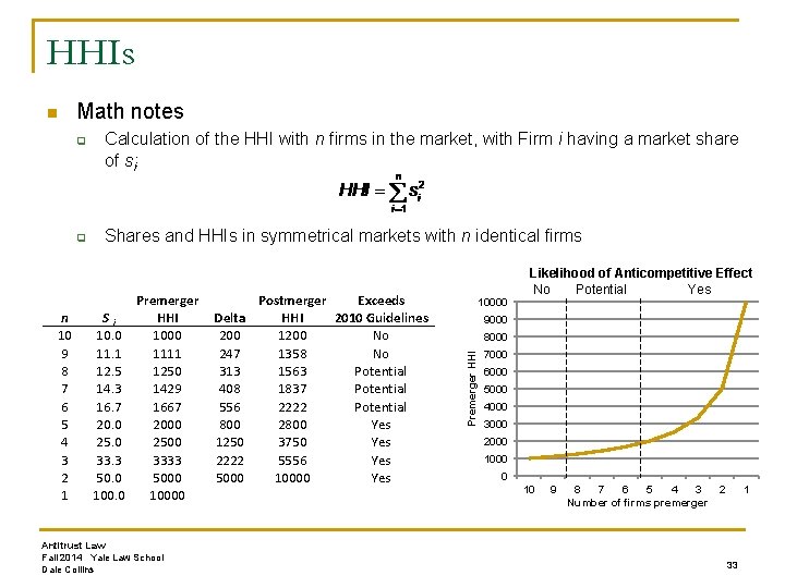
HHIs Math notes q q n 10 9 8 7 6 5 4 3 2 1 Calculation of the HHI with n firms in the market, with Firm i having a market share of si: Shares and HHIs in symmetrical markets with n identical firms Premerger Si HHI 10. 0 1000 11. 1 1111 12. 5 1250 14. 3 1429 16. 7 1667 20. 0 2000 2500 33. 3 3333 50. 0 5000 10000 Antitrust Law Fall 2014 Yale Law School Dale Collins Postmerger Exceeds Delta HHI 2010 Guidelines 200 1200 No 247 1358 No 313 1563 Potential 408 1837 Potential 556 2222 Potential 800 2800 Yes 1250 3750 Yes 2222 5556 Yes 5000 10000 Yes 10000 Likelihood of Anticompetitive Effect No Potential Yes 9000 8000 Premerger HHI n 7000 6000 5000 4000 3000 2000 1000 0 10 9 8 7 6 5 4 3 Number of firms premerger 2 1 33

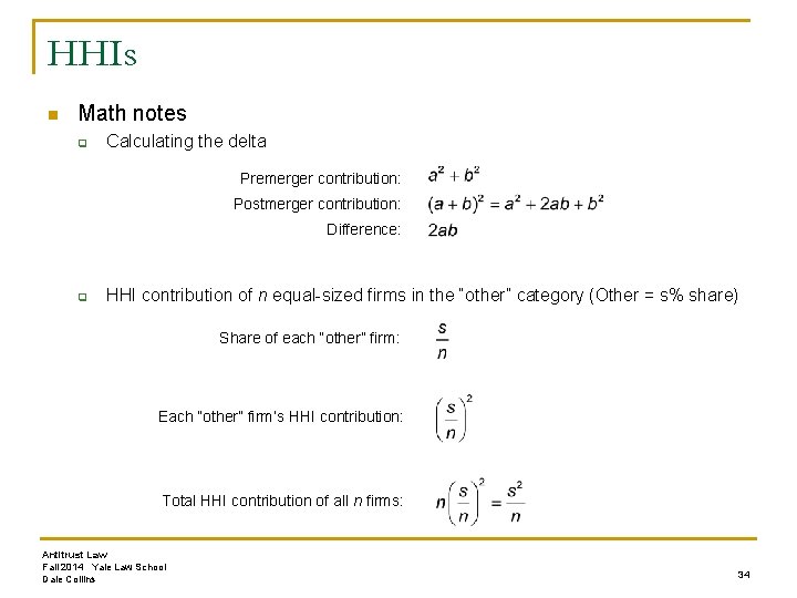
HHIs n Math notes q Calculating the delta Premerger contribution: Postmerger contribution: Difference: q HHI contribution of n equal-sized firms in the “other” category (Other = s% share) Share of each “other” firm: Each ”other” firm’s HHI contribution: Total HHI contribution of all n firms: Antitrust Law Fall 2014 Yale Law School Dale Collins 34

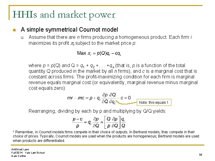
HHIs and market power n A simple symmetrical Cournot model q Assume that there are n firms producing a homogeneous product. Each firm i maximizes its profit i subject to the market price p: where p = p(Q) and Q = q 1 + q 2 +. . . +qn (that is, p is a function of the total quantity Q produced in the market by all n firms), and c is a marginal cost that is constant across firms. The profit-maximizing condition for each firm is marginal revenue equals marginal cost (or equivalently, marginal revenue minus marginal cost equals zero): Note: this equals 1 Rearranging, dividing by each by p and multiplying by Q/Q yields: Remember, in Cournot models firms compete in their choice of outputs. In Bertrand models, they compete in their choice of prices. Typically, Cournot models are used when the products are homogeneous; Bertrand models are used when products are differentiated. 1 Antitrust Law Fall 2014 Yale Law School Dale Collins 35

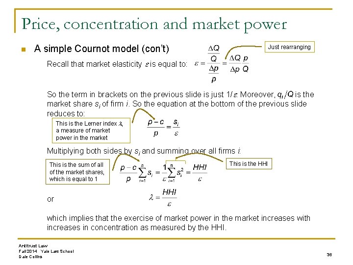
Price, concentration and market power n A simple Cournot model (con’t) Just rearranging Recall that market elasticity is equal to: So the term in brackets on the previous slide is just 1/. Moreover, is the market share si of firm i. So the equation at the bottom of the previous slide reduces to: This is the Lerner index , a measure of market power in the market Multiplying both sides by si and summing over all firms i: This is the sum of all of the market shares, which is equal to 1 This is the HHI or which implies that the exercise of market power in the market increases with increases in concentration as measured by the HHI. Antitrust Law Fall 2014 Yale Law School Dale Collins 36

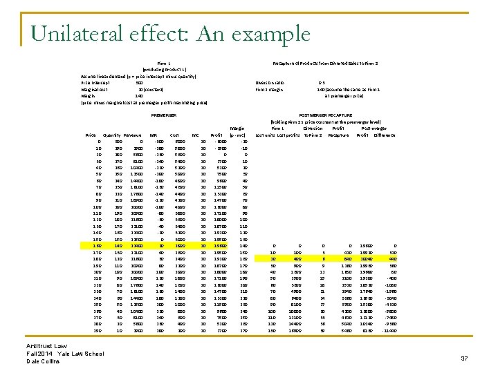
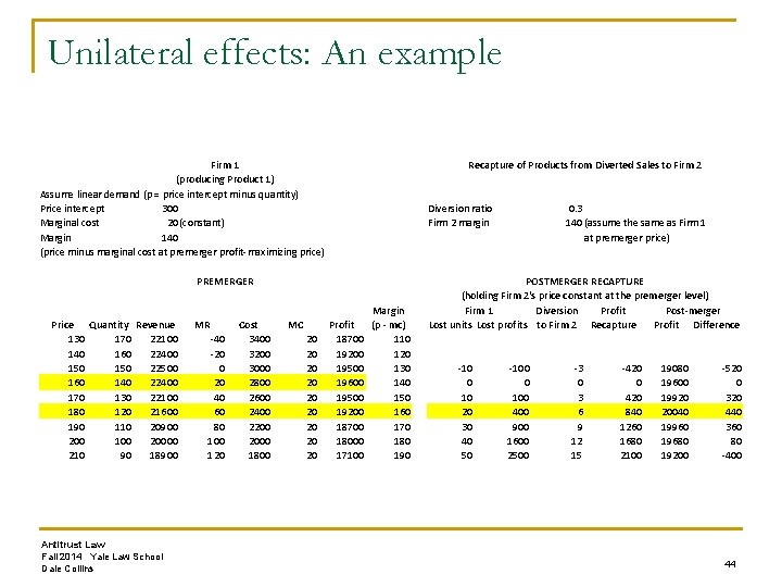
Unilateral effect: An example Firm 1 (producing Product 1) Assume linear demand (p = price intercept minus quantity) Price intercept 300 Marginal cost 20 (constant) Margin 140 (price minus marginal cost at premerger profit-maximizing price) Recapture of Products from Diverted Sales to Firm 2 Diversion ratio Firm 2 margin PREMERGER Price 0 10 20 30 40 50 60 70 80 90 100 110 120 130 140 150 160 170 180 190 200 210 220 230 240 250 260 270 280 290 Quantity Revenue 300 0 2900 280 5600 270 8100 260 10400 250 12500 240 14400 230 16100 220 17600 210 18900 20000 190 20900 180 21600 170 22100 160 22400 150 22500 140 22400 130 22100 120 21600 110 20900 100 20000 90 18900 80 17600 70 16100 60 14400 50 12500 40 10400 30 8100 20 5600 10 2900 Antitrust Law Fall 2014 Yale Law School Dale Collins MR -300 -280 -260 -240 -220 -200 -180 -160 -140 -120 -100 -80 -60 -40 -20 0 20 40 60 80 100 120 140 160 180 200 220 240 260 280 Cost 6000 5800 5600 5400 5200 5000 4800 4600 4400 4200 4000 3800 3600 3400 3200 3000 2800 2600 2400 2200 2000 1800 1600 1400 1200 1000 800 600 400 200 MC 20 20 20 20 20 20 20 20 Margin Profit (p - mc) -6000 -2900 -10 0 0 2700 10 5200 20 7500 30 9600 40 11500 50 13200 60 14700 70 16000 80 17100 90 18000 18700 110 19200 120 19500 130 19600 140 19500 150 19200 160 18700 170 18000 180 17100 190 16000 200 14700 210 13200 220 11500 230 9600 240 7500 250 5200 260 270 0. 3 140 (assume the same as Firm 1 at premerger price) POSTMERGER RECAPTURE (holding Firm 2's price constant at the premerger level) Firm 1 Diversion Profit Post-merger Lost units Lost profits to Firm 2 Recapture Profit Difference 0 10 20 30 40 50 60 70 80 90 100 110 120 130 0 100 400 900 1600 2500 3600 4900 6400 8100 10000 12100 14400 16900 0 3 6 9 12 15 18 21 24 27 30 33 36 39 0 420 840 1260 1680 2100 2520 2940 3360 3780 4200 4620 5040 5460 19600 19920 20040 19960 19680 19200 18520 17640 16560 15280 13800 12120 10240 8160 0 320 440 360 80 -400 -1080 -1960 -3040 -4320 -5800 -7480 -9360 -11440 37

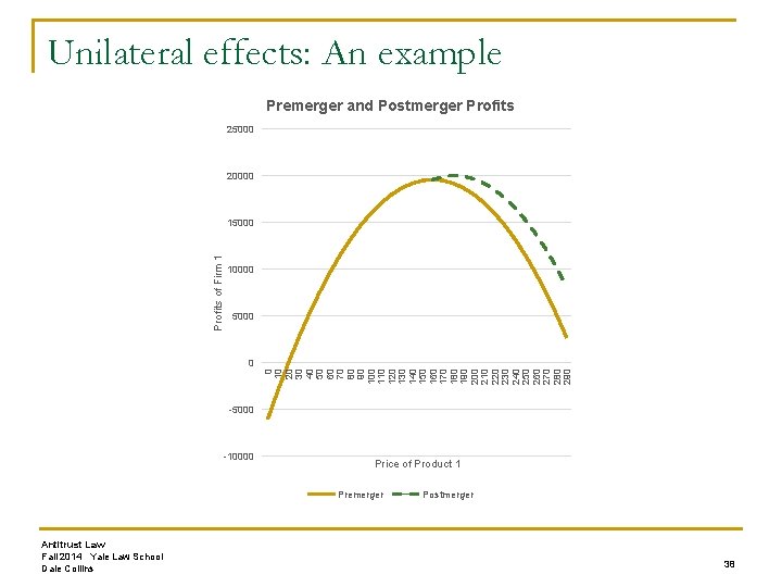
Unilateral effects: An example Premerger and Postmerger Profits 25000 20000 Profits of Firm 1 15000 10000 5000 0 10 20 30 40 50 60 70 80 90 100 110 120 130 140 150 160 170 180 190 200 210 220 230 240 250 260 270 280 290 0 -5000 -10000 Price of Product 1 Premerger Antitrust Law Fall 2014 Yale Law School Dale Collins Postmerger 38

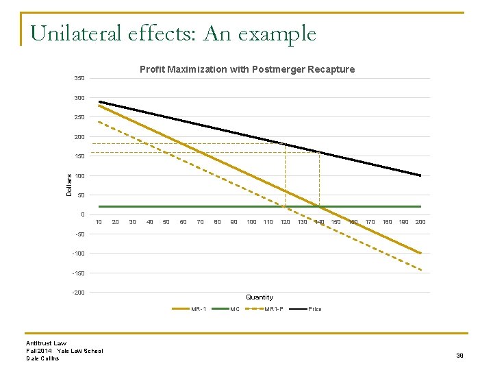
Unilateral effects: An example Profit Maximization with Postmerger Recapture 350 300 250 200 Dollars 150 100 50 0 10 20 30 40 50 60 70 80 90 100 110 120 130 140 150 160 170 180 190 200 -50 -100 -150 -200 Quantity MR-1 Antitrust Law Fall 2014 Yale Law School Dale Collins MC MR 1 -P Price 39

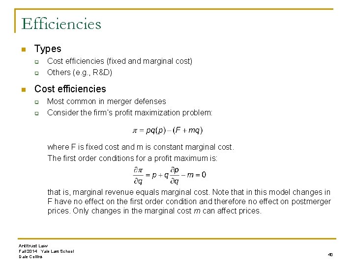
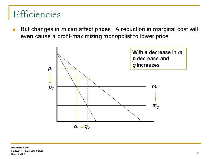
Efficiencies n Types q q n Cost efficiencies (fixed and marginal cost) Others (e. g. , R&D) Cost efficiencies q q Most common in merger defenses Consider the firm’s profit maximization problem: where F is fixed cost and m is constant marginal cost. The first order conditions for a profit maximum is: that is, marginal revenue equals marginal cost. Note that in this model changes in F have no effect on the first order condition and therefore no effect on postmerger prices. Only changes in the marginal cost m can affect prices. Antitrust Law Fall 2014 Yale Law School Dale Collins 40

Efficiencies n But changes in m can affect prices. A reduction in marginal cost will even cause a profit-maximizing monopolist to lower price. With a decrease in m, p decrease and q increases p 1 m 1 p 2 m 2 q 1 Antitrust Law Fall 2014 Yale Law School Dale Collins q 2 41

Antitrust Law Fall 2014 Yale Law School Dale Collins 42

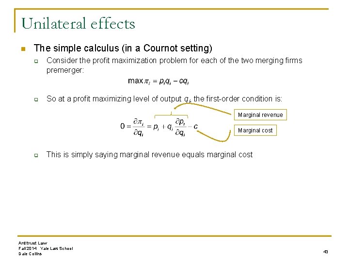
Unilateral effects n The simple calculus (in a Cournot setting) q q Consider the profit maximization problem for each of the two merging firms premerger: So at a profit maximizing level of output qi, the first-order condition is: Marginal revenue Marginal cost q This is simply saying marginal revenue equals marginal cost Antitrust Law Fall 2014 Yale Law School Dale Collins 43

Unilateral effects: An example Firm 1 (producing Product 1) Assume linear demand (p = price intercept minus quantity) Price intercept 300 Marginal cost 20 (constant) Margin 140 (price minus marginal cost at premerger profit-maximizing price) Recapture of Products from Diverted Sales to Firm 2 Diversion ratio Firm 2 margin PREMERGER Price Quantity Revenue 130 170 22100 140 160 22400 150 22500 160 140 22400 170 130 22100 180 120 21600 190 110 20900 200 100 20000 210 90 18900 Antitrust Law Fall 2014 Yale Law School Dale Collins MR -40 -20 0 20 40 60 80 100 120 Cost 3400 3200 3000 2800 2600 2400 2200 2000 1800 MC 20 20 20 Margin Profit (p - mc) 18700 110 19200 120 19500 130 19600 140 19500 150 19200 160 18700 170 18000 180 17100 190 0. 3 140 (assume the same as Firm 1 at premerger price) POSTMERGER RECAPTURE (holding Firm 2's price constant at the premerger level) Firm 1 Diversion Profit Post-merger Lost units Lost profits to Firm 2 Recapture Profit Difference -10 0 10 20 30 40 50 -100 0 100 400 900 1600 2500 -3 0 3 6 9 12 15 -420 0 420 840 1260 1680 2100 19080 19600 19920 20040 19960 19680 19200 -520 0 320 440 360 80 -400 44