Economics 387 Lecture 8 Consumer Choice and Demand

Economics 387 Lecture 8 Consumer Choice and Demand Tianxu Chen

Outline • Applying The Standard Budget Constraint Model • Two Additional Demand Shifters—Time and Coinsurance • Issues in Measuring Health Care Demand • Empirical Measurements of Demand Elasticities • Impacts of Insurance on Aggregate Expenditures • Other Variables Affecting Demand • Conclusions

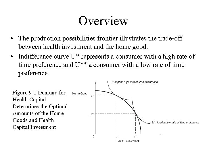
Overview • The production possibilities frontier illustrates the trade-off between health investment and the home good. • Indifference curve U* represents a consumer with a high rate of time preference and U** a consumer with a low rate of time preference. Figure 9 -1 Demand for Health Capital Determines the Optimal Amounts of the Home Goods and Health Capital Investment

Applying the Standard Budget Constraint Model • Model assumptions – – Consumer is rational and perfectly informed – There is no uncertainty about the future – Important decisions are made as if the future were known with certainty

Logic of Consumer Choice • Consumers can choose any affordable combination or bundle of goods, and from among these affordable bundles, they will choose the one preferred. • The depiction of this choice requires two elements: – The consumer’s preferences—described by a set of indifference curves – The consumer’s budget constraint—described by the straight budget line

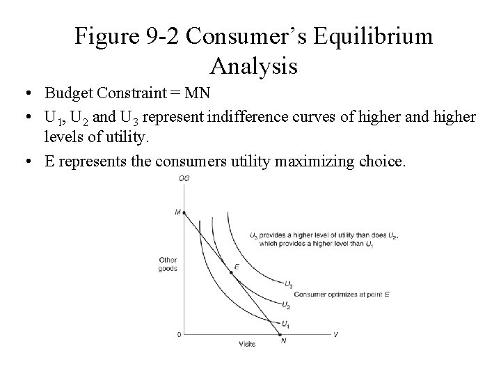
Figure 9 -2 Consumer’s Equilibrium Analysis • Budget Constraint = MN • U 1, U 2 and U 3 represent indifference curves of higher and higher levels of utility. • E represents the consumers utility maximizing choice.

Utility Maximization • At point E the slope of indifference curve U 2 (marginal rate of substitution) is just equal to the price ratio PV/POG. • The marginal rate of substitution (MRS) is a measure of the rate at which a consumer is willing to trade other goods for physician visits and the price ratio is a measure of the rate at which she can trade other goods for physician visits.

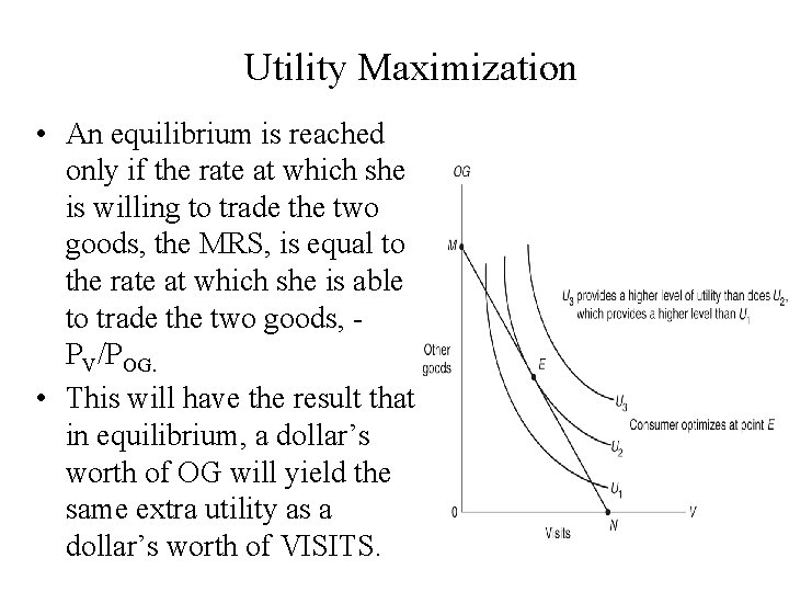
Utility Maximization • An equilibrium is reached only if the rate at which she is willing to trade the two goods, the MRS, is equal to the rate at which she is able to trade the two goods, PV/POG. • This will have the result that in equilibrium, a dollar’s worth of OG will yield the same extra utility as a dollar’s worth of VISITS.

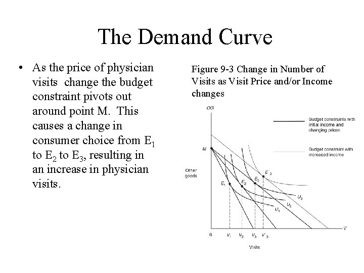
The Demand Curve • As the price of physician visits change the budget constraint pivots out around point M. This causes a change in consumer choice from E 1 to E 2 to E 3, resulting in an increase in physician visits. Figure 9 -3 Change in Number of Visits as Visit Price and/or Income changes

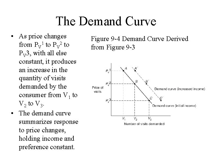
The Demand Curve • As price changes from PV 1 to PV 2 to PV 3, with all else constant, it produces an increase in the quantity of visits demanded by the consumer from V 1 to V 2 to V 3. • The demand curve summarizes response to price changes, holding income and preference constant. Figure 9 -4 Demand Curve Derived from Figure 9 -3

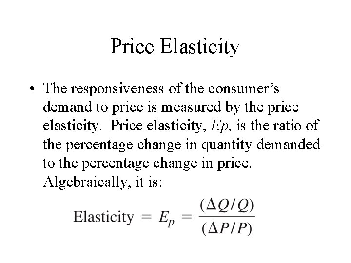
Price Elasticity • The responsiveness of the consumer’s demand to price is measured by the price elasticity. Price elasticity, Ep, is the ratio of the percentage change in quantity demanded to the percentage change in price. Algebraically, it is:

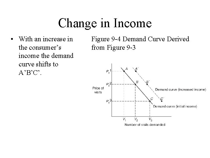
Change in Income • With an increase in the consumer’s income the demand curve shifts to A’B’C’. Figure 9 -4 Demand Curve Derived from Figure 9 -3

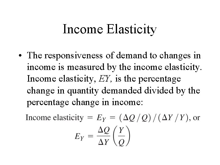
Income Elasticity • The responsiveness of demand to changes in income is measured by the income elasticity. Income elasticity, EY, is the percentage change in quantity demanded divided by the percentage change in income:

Changes in the Price of Substitutes and Complements • One would expect that increases in the prices of substitutes to physician visits (hospital outpatient services, visits to other providers) would increase the demand for office visits. In other words, an increase in the price of a substitute will shift the demand curve to the right. Increases in the prices of complements (diagnostic services) would reduce demand for office visits.

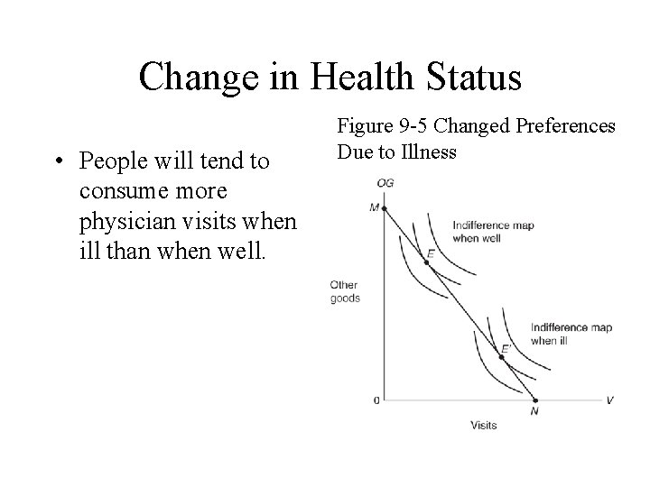
Change in Health Status • People will tend to consume more physician visits when ill than when well. Figure 9 -5 Changed Preferences Due to Illness

TWO ADDITIONAL DEMAND SHIFTERSTIME AND COINSURANCE • The analysis thus far suggests that price, income level, tastes, health status, and other circumstances influence the consumption of physician services. • However, other considerations, the roles of insurance and of time, cannot be overlooked.

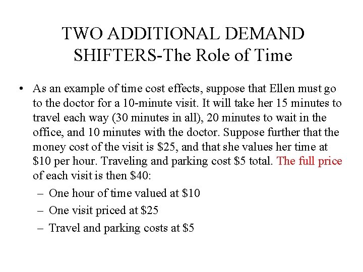
TWO ADDITIONAL DEMAND SHIFTERS-The Role of Time • As an example of time cost effects, suppose that Ellen must go to the doctor for a 10 -minute visit. It will take her 15 minutes to travel each way (30 minutes in all), 20 minutes to wait in the office, and 10 minutes with the doctor. Suppose further that the money cost of the visit is $25, and that she values her time at $10 per hour. Traveling and parking cost $5 total. The full price of each visit is then $40: – One hour of time valued at $10 – One visit priced at $25 – Travel and parking costs at $5

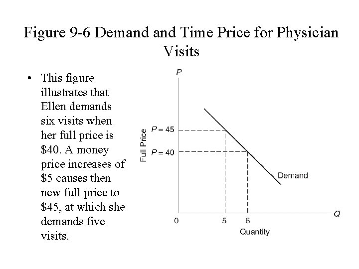
Figure 9 -6 Demand Time Price for Physician Visits • This figure illustrates that Ellen demands six visits when her full price is $40. A money price increases of $5 causes then new full price to $45, at which she demands five visits.

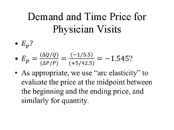
Demand Time Price for Physician Visits •

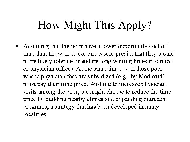
How Might This Apply? • Assuming that the poor have a lower opportunity cost of time than the well-to-do, one would predict that they would more likely tolerate or endure long waiting times in clinics or physician offices. At the same time, even those poor whose physician fees are subsidized (e. g. , by Medicaid) must pay their time price. Wishing to increase physician visits among the poor, we might choose to reduce the time price by building nearby clinics and expanding outreach programs, a strategy that has been developed in many localities.

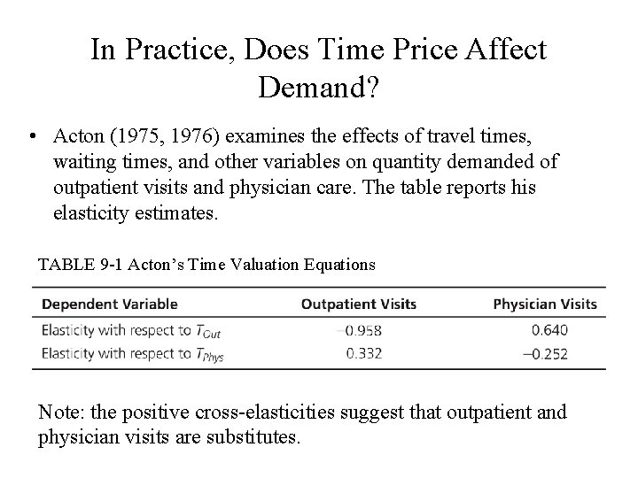
In Practice, Does Time Price Affect Demand? • Acton (1975, 1976) examines the effects of travel times, waiting times, and other variables on quantity demanded of outpatient visits and physician care. The table reports his elasticity estimates. TABLE 9 -1 Acton’s Time Valuation Equations Note: the positive cross-elasticities suggest that outpatient and physician visits are substitutes.

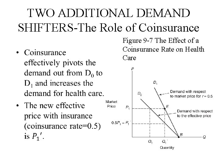
TWO ADDITIONAL DEMAND SHIFTERS-The Role of Coinsurance • Figure 9 -7 The Effect of a Coinsurance Rate on Health Care

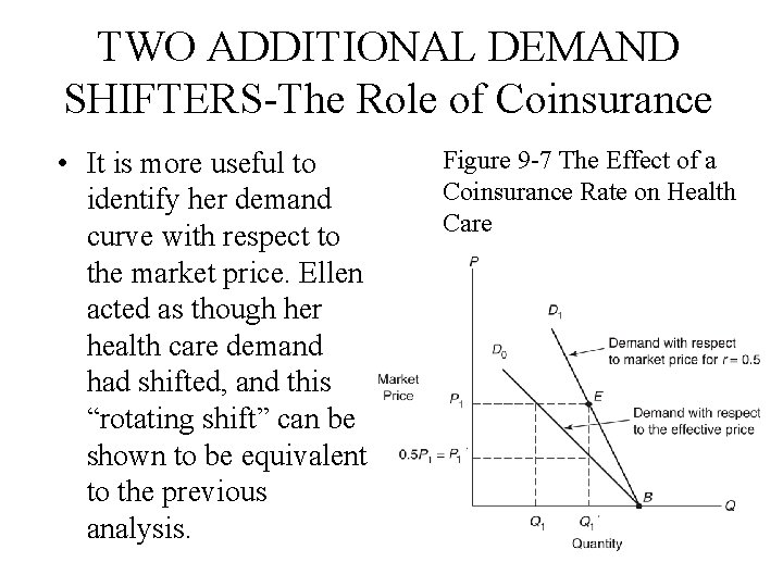
TWO ADDITIONAL DEMAND SHIFTERS-The Role of Coinsurance • It is more useful to identify her demand curve with respect to the market price. Ellen acted as though her health care demand had shifted, and this “rotating shift” can be shown to be equivalent to the previous analysis. Figure 9 -7 The Effect of a Coinsurance Rate on Health Care

TWO ADDITIONAL DEMAND SHIFTERS-The Role of Coinsurance • The exercise makes two theoretical facts clearer: 1. Insurance will increase consumer’s demand for health care; 2. and insurance will make consumer’s demand for health care less elastic.

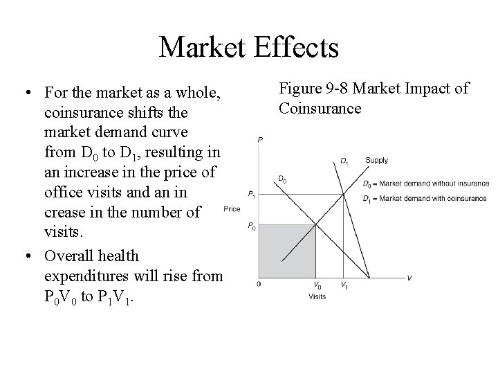
Market Effects • For the market as a whole, coinsurance shifts the market demand curve from D 0 to D 1, resulting in an increase in the price of office visits and an in crease in the number of visits. • Overall health expenditures will rise from P 0 V 0 to P 1 V 1. Figure 9 -8 Market Impact of Coinsurance

ISSUES IN MEASURING HEALTH CARE DEMAND Overview • In this section, the focus is on variables of interest to science and public policy. • We examine how health care demand responds to money price, insurance coverage, and time price. • In addition, we examine the effects on market demand of income and other variables. • We identify FIVE issues.

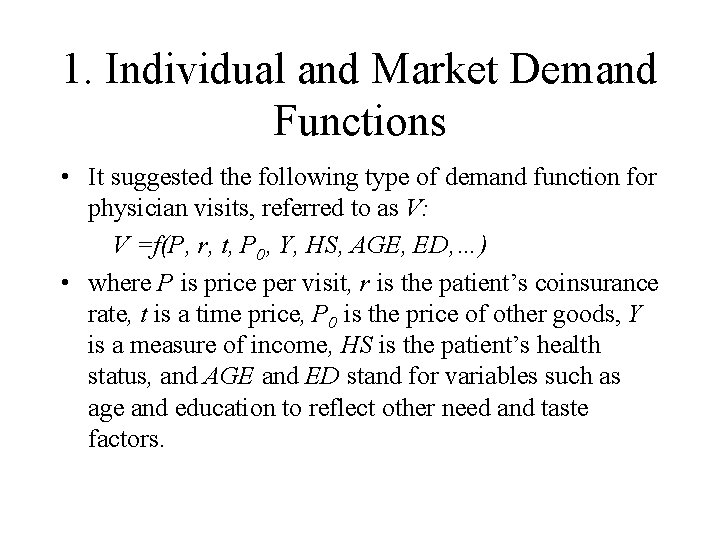
1. Individual and Market Demand Functions • It suggested the following type of demand function for physician visits, referred to as V: V =f(P, r, t, P 0, Y, HS, AGE, ED, …) • where P is price per visit, r is the patient’s coinsurance rate, t is a time price, P 0 is the price of other goods, Y is a measure of income, HS is the patient’s health status, and AGE and ED stand for variables such as age and education to reflect other need and taste factors.

2. Measurement and Definitions • There alternative definitions of health care quantities, as well as alternative measuring tools. • Investigators often measure the quantity of services in dollar expenditures. One problem is that expenditures reflect a complex combination of price of care, quantities of care, and qualities of care. • Alternative measures include quantity of visits, patient days, or cases treated, yet these do not necessarily measure the intensity of care. • A related problem is to define the price of services. Because of the prevalence of health insurance, most patients do not pay the full price for their treatments.

3. Differences in Study Populations • Different researchers, naturally, use different samples or populations. • Elasticities will differ between populations and even within populations at different points in time. • For example, many health economists believe that income elasticities for health care have become smaller over the years in the United States, presumably because of the effects of programs like Medicare and Medicaid.

4. Data Sources • A common source of health care data is the insurance claim. Claims data, however, are limited to services covered by insurance and used by the insured. Furthermore, claims data often lack detail on individuals’ characteristics, such as education and income. • In contrast, health interview survey data often incorporate personal data, but their accuracy depends on the recall ability of the people being interviewed.

5. Experimental and Nonexperimental Data • Much of health care demand research used nonexperimental data, and thus the researcher could not control the environment or assure that other extraneous variables were held constant. • A useful alternative involving the natural experiment is sometimes possible. A natural experiment, for example, may occur when a given area changes its health insurance plan.

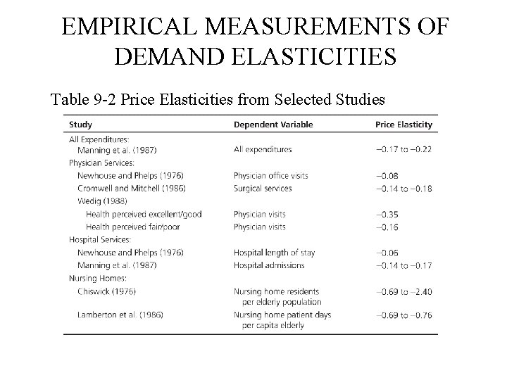
EMPIRICAL MEASUREMENTS OF DEMAND ELASTICITIES Table 9 -2 Price Elasticities from Selected Studies

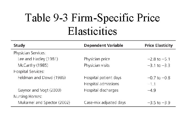
Table 9 -3 Firm-Specific Price Elasticities

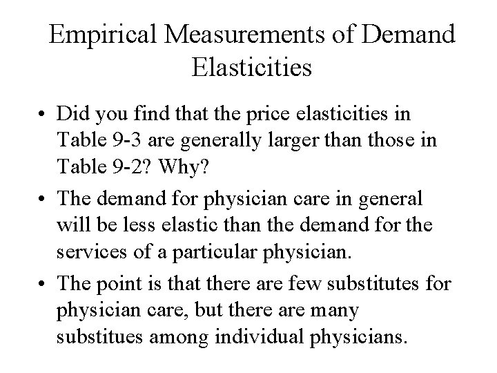
Empirical Measurements of Demand Elasticities • Did you find that the price elasticities in Table 9 -3 are generally larger than those in Table 9 -2? Why? • The demand for physician care in general will be less elastic than the demand for the services of a particular physician. • The point is that there are few substitutes for physician care, but there are many substitues among individual physicians.

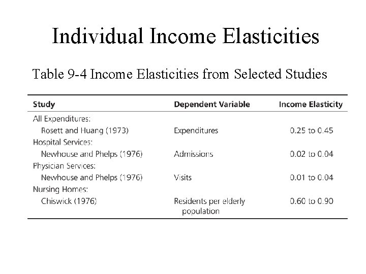
Individual Income Elasticities Table 9 -4 Income Elasticities from Selected Studies

Income Elasticities Across Countries • An early cross-national study published by Newhouse (1977) found elasticity estimates ranging from 1. 15 to 1. 31. • Parkin and colleagues (1987) pointed out several potential weaknesses in most existing crossnational studies, but despite their objections, offered improved results that tended to support the finding of cross-national income elasticities greater than 1. 0. • Gerdtham et al. (1992) and Getzen and Poullier (1992) also lend support to the result.

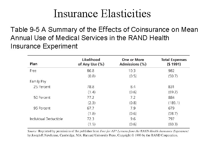
Insurance Elasticities Table 9 -5 A Summary of the Effects of Coinsurance on Mean Annual Use of Medical Services in the RAND Health Insurance Experiment

IMPACTS OF INSURANCE ON AGGREGATE EXPENDITURES Summary • According to the RAND investigators, coinsurance and income accounted for about one-fifth of the total increase in real health expenditures. • Subsequent research (Peden and Freeland, 1998) determined that about half of the expenditure increase was due to induced technological innovation.

OTHER VARIABLES AFFECTING DEMAND Ethnicity and Gender • Many studies of demand examine the influence of race, and find that blacks tend to consume less medical care than the other large, self-identified ethnic groups when other factors are held constant. • Females differ from males most clearly in their time pattern of medical care usage. During childbearing years, women are relatively heavy users of health care, but women are healthier in the long run and they predominate in the numbers of the elderly.

Urban vs. Rural • Studies sometimes find differences in health care usage due to rural status. If rural residents use less care, the reasons why are not necessarily clear. Rural dwellers may differ culturally, and some analysts argue that this factor is more important to one’s perception of life than ethnicity is.

Education • Education is strongly associated with better health. If you are a college student, the odds are very good that you are healthier than your non-college counterparts. As in the demand for health capital model, this may be because you are a more efficient producer of health, you are less likely to smoke, and you are more likely to eat a healthful diet.

Age, Health Status and Uncertainty • Older people consume three to four times more health care than the younger population. • Wedig (1988) finds that the price elasticity of the decision to seek health care tends to be lower in absolute value for those with poorer health status, regardless of which measure is used to record health status. • Finally, uncertainty will affect health care demand. When a consumer, worried about a future health risk, seeks advice or preventive treatment, we call this a precautionary demand (Picone, Uribe, and Wilson, 1998).

CONCLUSIONS • Demand theory is crucial to our understanding of health care markets. • The substantial increases in out-of-pocket costs for prescription products experienced by many patients have affected utilization of drugs in the expected negative direction. • Time and distance can also be important as theory suggests.

CONCLUSIONS • An analysis of the demand for physician care in 12 European Union countries illustrates the universal relevance of demand theory. Jiménez-Martin and colleagues (2004) show that one-third to one-half the variability in demand across countries is explained by differences in age, income, and the physician’s role in the health care system

CONCLUSIONS • Finally, a good understanding of demand theory serves as the rationale for marketbased, consumer-driven approaches to health system reform.