Chapter 21 Theory of Consumer Choice Ratna K

Chapter 21 Theory of Consumer Choice Ratna K. Shrestha

Theory of Consumer Choice. . . addresses the following questions and links them in understanding: Ø Ø Ø How do wages affect labor supply? How do interest rates affect household saving? Do the poor prefer to receive cash or in-kind transfers?

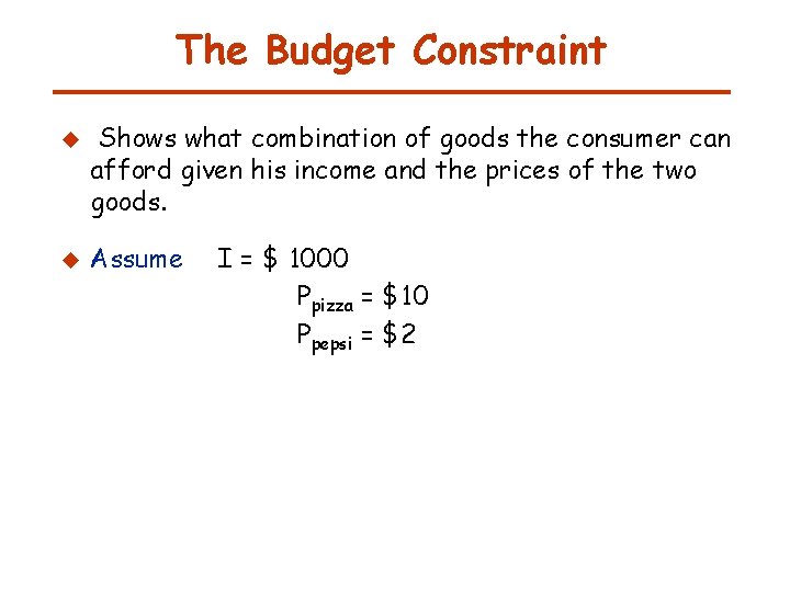
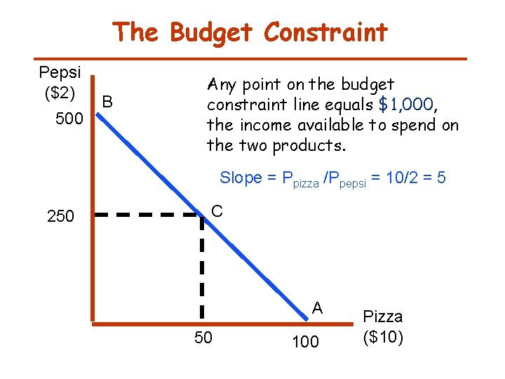
The Budget Constraint u u Shows what combination of goods the consumer can afford given his income and the prices of the two goods. Assume I = $ 1000 Ppizza = $10 Ppepsi = $2

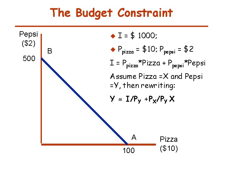
The Budget Constraint Pepsi ($2) 500 B u I = $ 1000; u Ppizza = $10; Ppepsi = $2 I = Ppizza*Pizza + Ppepsi*Pepsi Assume Pizza =X and Pepsi =Y, then rewriting: Y = I/PY +PX/PY X A 100 Pizza ($10)

The Budget Constraint Pepsi ($2) 500 B Any point on the budget constraint line equals $1, 000, the income available to spend on the two products. Slope = Ppizza /Ppepsi = 10/2 = 5 250 C A 50 100 Pizza ($10)

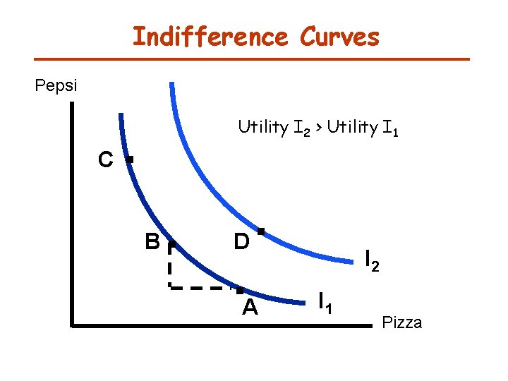
Preferences 1. 2. 3. 4. Indifference curves illustrate consumer’s preference between different bundles of goods and services. An indifference curve depicts bundles of goods that make the consumer equally well-off. It shows the combinations of goods that give the consumer the same level of utility. In the next slide, the levels of utility that the consumer can derive from three bundles A or B or C, which are on the same curve, are equal. The bundle D provides higher utility than bundle A, B or C.

Indifference Curves Pepsi C . Utility I 2 > Utility I 1 B . . . D A I 2 I 1 Pizza

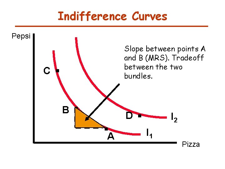
Indifference Curves Pepsi C . B . Slope between points A and B (MRS). Tradeoff between the two bundles. . . D A I 2 I 1 Pizza

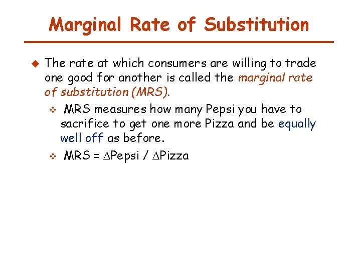
Marginal Rate of Substitution u The rate at which consumers are willing to trade one good for another is called the marginal rate of substitution (MRS). v MRS measures how many Pepsi you have to sacrifice to get one more Pizza and be equally well off as before. v MRS = Pepsi / Pizza

Properties of Indifference Curves Higher indifference curves are preferred to lower ones. Indifference curves are downward sloping. Indifference curves do not cross. Indifference curves are bowed inward.

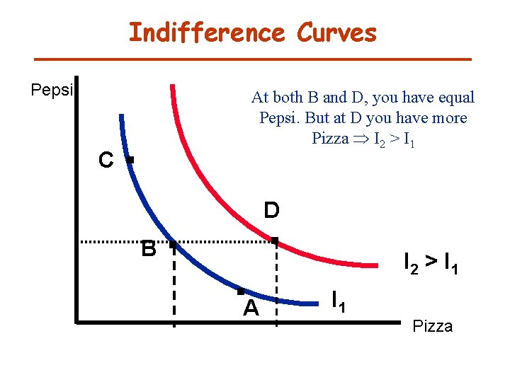
Properties of Indifference Curves (1) Higher indifference curves are preferred to lower ones Ø Ø Because consumers prefer more consumption to less, higher indifference curves are preferred to lower ones. Indifference curves farther from the origin represent higher levels of well-being or utility.

Indifference Curves Pepsi C . At both B and D, you have equal Pepsi. But at D you have more Pizza I 2 > I 1 . . . D B A I 2 > I 1 Pizza

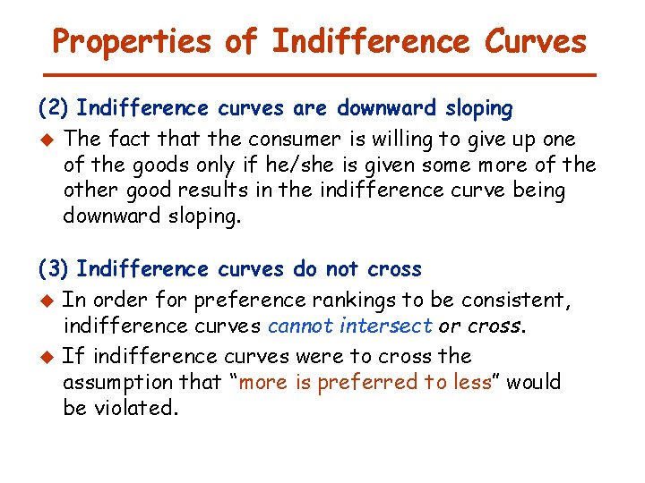
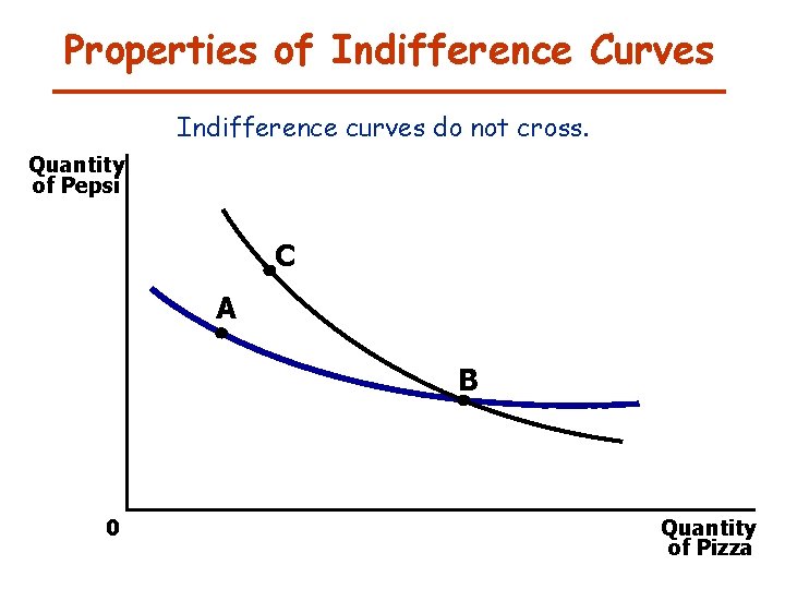
Properties of Indifference Curves (2) Indifference curves are downward sloping u The fact that the consumer is willing to give up one of the goods only if he/she is given some more of the other good results in the indifference curve being downward sloping. (3) Indifference curves do not cross u In order for preference rankings to be consistent, indifference curves cannot intersect or cross. u If indifference curves were to cross the assumption that “more is preferred to less” would be violated.

Properties of Indifference Curves Indifference curves do not cross. Quantity of Pepsi C A B 0 Quantity of Pizza

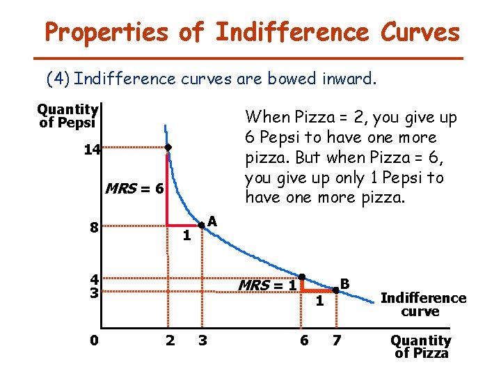
Properties of Indifference Curves (4) Indifference curves are bowed inward. Quantity of Pepsi When Pizza = 2, you give up 6 Pepsi to have one more pizza. But when Pizza = 6, you give up only 1 Pepsi to have one more pizza. 14 MRS = 6 8 A 1 4 3 0 MRS = 1 2 3 1 6 B 7 Indifference curve Quantity of Pizza

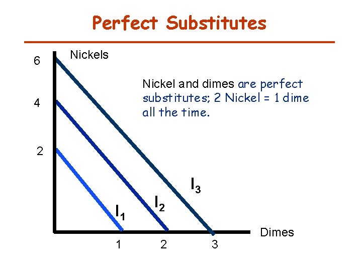
Perfect Substitutes 6 Nickels Nickel and dimes are perfect substitutes; 2 Nickel = 1 dime all the time. 4 2 I 1 1 I 2 2 I 3 3 Dimes

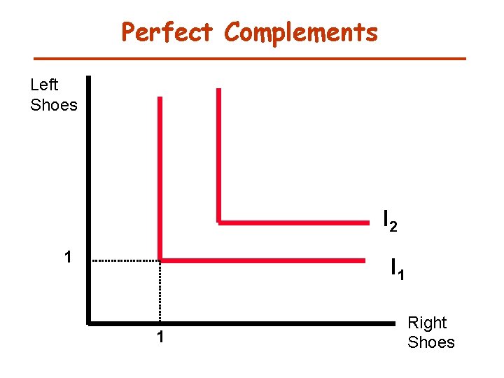
Perfect Complements Left Shoes I 2 1 I 1 1 Right Shoes

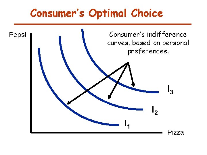
Consumer’s Optimal Choice Pepsi Consumer’s indifference curves, based on personal preferences. I 3 I 2 I 1 Pizza

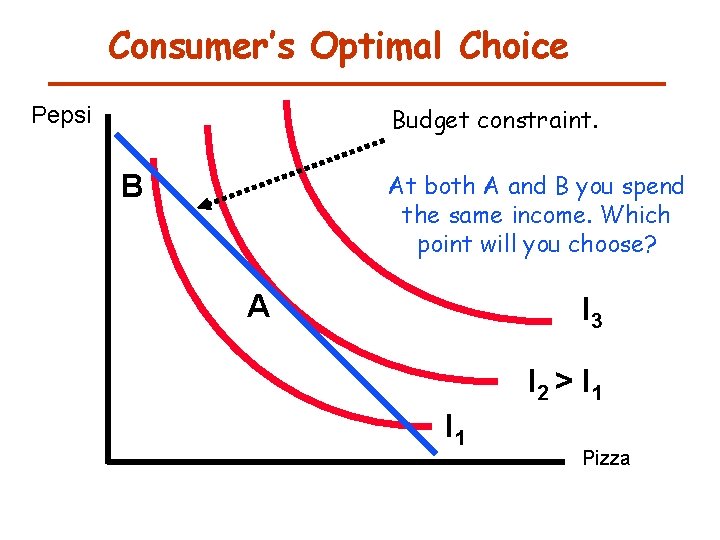
Consumer’s Optimal Choice Pepsi Budget constraint. B At both A and B you spend the same income. Which point will you choose? A I 3 I 2 > I 1 Pizza

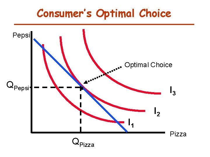
Consumer’s Optimal Choice Pepsi QPepsi . Optimal Choice I 3 I 1 QPizza I 2 Pizza

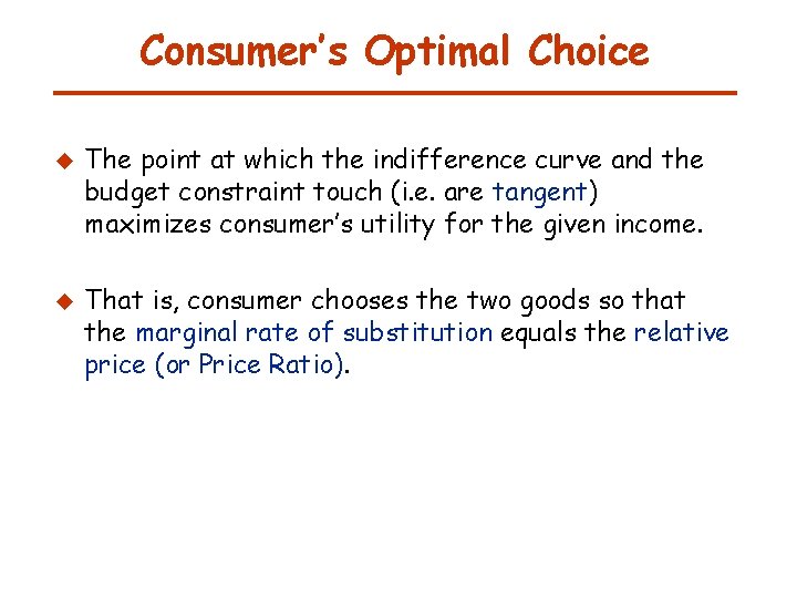
Consumer’s Optimal Choice u u The point at which the indifference curve and the budget constraint touch (i. e. are tangent) maximizes consumer’s utility for the given income. That is, consumer chooses the two goods so that the marginal rate of substitution equals the relative price (or Price Ratio).

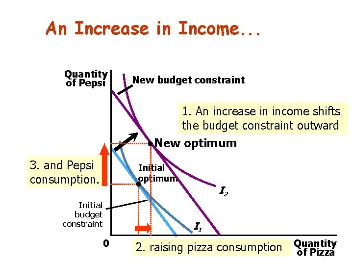
An Increase in Income. . . Quantity of Pepsi New budget constraint 1. An increase in income shifts the budget constraint outward New optimum 3. and Pepsi consumption. Initial optimum I 2 Initial budget constraint I 1 0 2. raising pizza consumption Quantity of Pizza

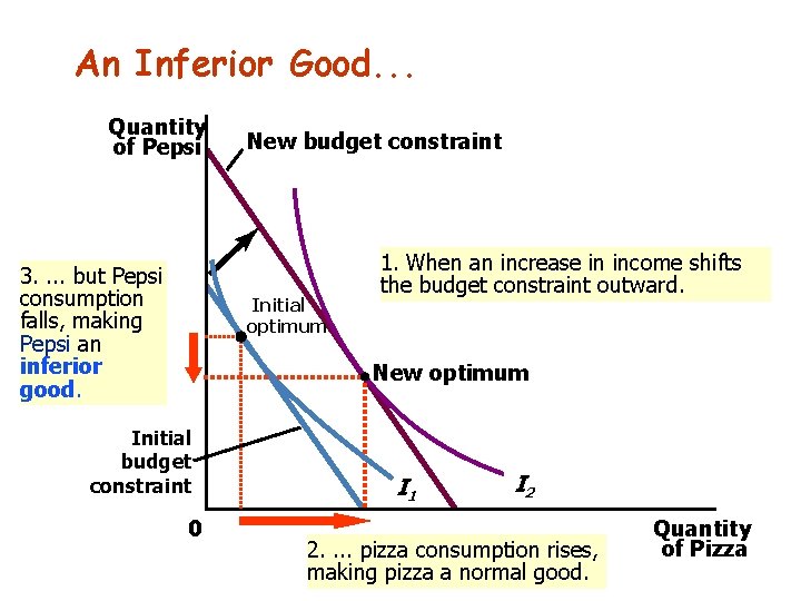
An Inferior Good. . . Quantity of Pepsi 3. . but Pepsi consumption falls, making Pepsi an inferior good. New budget constraint Initial optimum 1. When an increase in income shifts the budget constraint outward. New optimum Initial budget constraint 0 I 1 I 2 2. . pizza consumption rises, making pizza a normal good. Quantity of Pizza

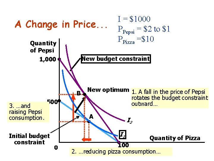
A Change in Price. . . Quantity of Pepsi 1, 000 New budget constraint B 3. …and raising Pepsi consumption. 500 Initial budget constraint I = $1000 PPepsi = $2 to $1 PPizza =$10 New optimum 1. A fall in the price of Pepsi rotates the budget constraint outward… A I 2 I 1 0 Quantity of Pizza 100 2. …reducing pizza consumption…

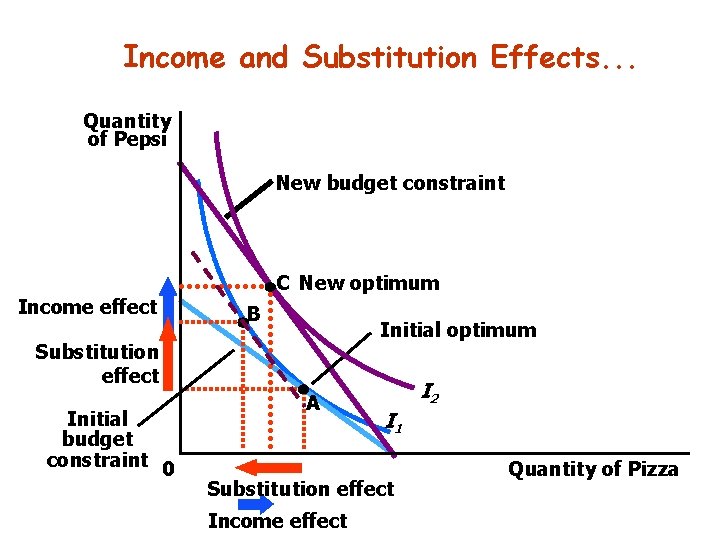
Income and Substitution Effects u v v The price effect can be divided into: an income effect a substitution effect

Income and Substitution Effects. . . Quantity of Pepsi New budget constraint C New optimum Income effect B Initial optimum Substitution effect Initial budget constraint 0 A I 2 I 1 Substitution effect Income effect Quantity of Pizza

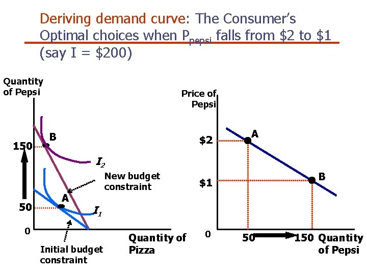
Deriving demand curve: The Consumer’s Optimal choices when Ppepsi falls from $2 to $1 (say I = $200) Quantity of Pepsi 150 Price of Pepsi B $2 A I 2 50 A New budget constraint B $1 I 1 0 Initial budget constraint Quantity of Pizza 0 50 150 Quantity of Pepsi

Applications: (1) How do increase in wages affect labor supply?

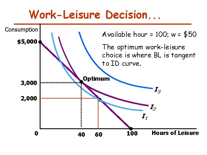
Work-Leisure Decision. . . Consumption Available hour = 100; w = $50 $5, 000 3, 000 The optimum work-leisure choice is where BL is tangent to ID curve. Optimum I 3 2, 000 I 2 I 1 0 40 60 100 Hours of Leisure

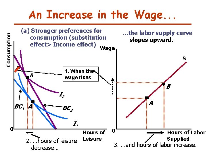
Consumption An Increase in the Wage. . . (a) Stronger preferences for consumption (substitution effect> Income effect) …the labor supply curve slopes upward. Wage S 1. When the wage rises B B I 2 BC 1 A 0 A BC 2 I 1 2. …hours of leisure decrease… Hours of Leisure 0 Hours of Labor Supplied 3. . and hours of labor increase.

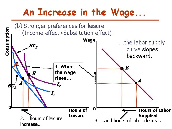
Consumption An Increase in the Wage. . . (b) Stronger preferences for leisure (Income effect>Substitution effect) Wage BC 2 1. When the wage rises… B BC 1 A . . the labor supply curve slopes backward. B A I 2 I 1 0 2. …hours of leisure increase… Hours of Leisure 0 Hours of Labor Supplied 3. . and hours of labor decrease.

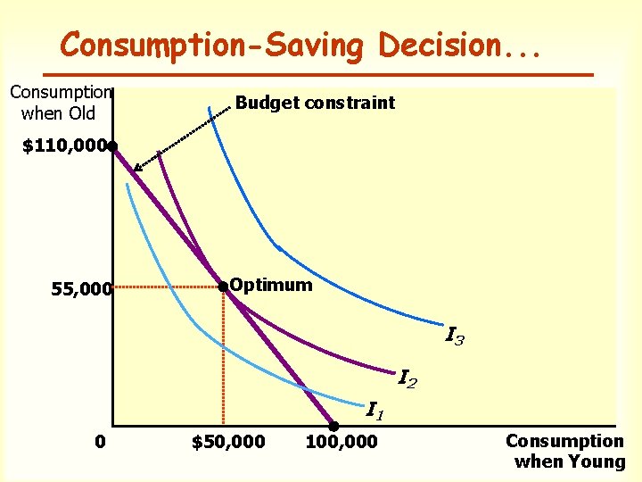
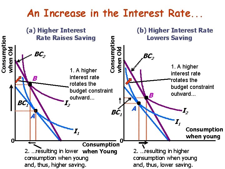
(2) How do interest rates affect household saving? u An increase in the interest rate could either encourage or discourage saving.

Consumption-Saving Decision. . . Consumption when Old Budget constraint $110, 000 55, 000 Optimum I 3 I 2 I 1 0 $50, 000 100, 000 Consumption when Young

(a) Higher Interest Rate Raises Saving BC 2 B BC 1 BC 2 1. A higher interest rate rotates the budget constraint outward. . . B I 2 BC 1 A 1. A higher interest rate rotates the budget constraint outward. . . A I 2 I 1 0 (b) Higher Interest Rate Lowers Saving Consumption when Old An Increase in the Interest Rate. . . Consumption 2. …resulting in lower when Young consumption when young and, thus, higher saving. 0 Consumption when young 2. …resulting in higher consumption when young and, thus, lower saving.

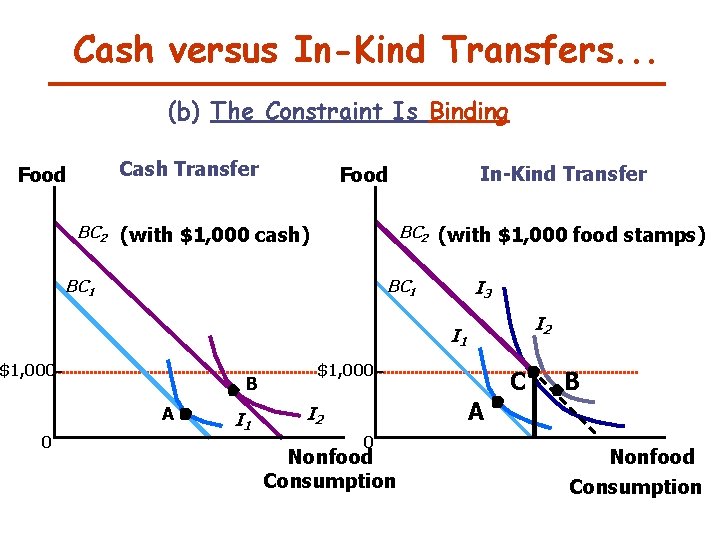
(3) Cash Vs. In Kind Transfer

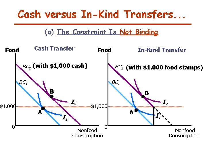
Cash versus In-Kind Transfers. . . (a) The Constraint Is Not Binding Cash Transfer Food In-Kind Transfer Food BC 2 (with $1, 000 cash) BC 2 (with $1, 000 food stamps) BC 1 B $1, 000 0 B I 2 A $1, 000 I 1 Nonfood Consumption 0 I 2 A I 1 Nonfood Consumption

Cash versus In-Kind Transfers. . . (b) The Constraint Is Binding Cash Transfer Food In-Kind Transfer Food BC 2 (with $1, 000 cash) BC 2 (with $1, 000 food stamps) BC 1 I 3 BC 1 I 2 I 1 $1, 000 B A 0 I 1 $1, 000 C B A I 2 0 Nonfood Consumption