ECE 472572 Lecture 11 Image Compression Fundamentals and

ECE 472/572 - Lecture 11 Image Compression – Fundamentals and Lossless Compression Techniques 11/03/11

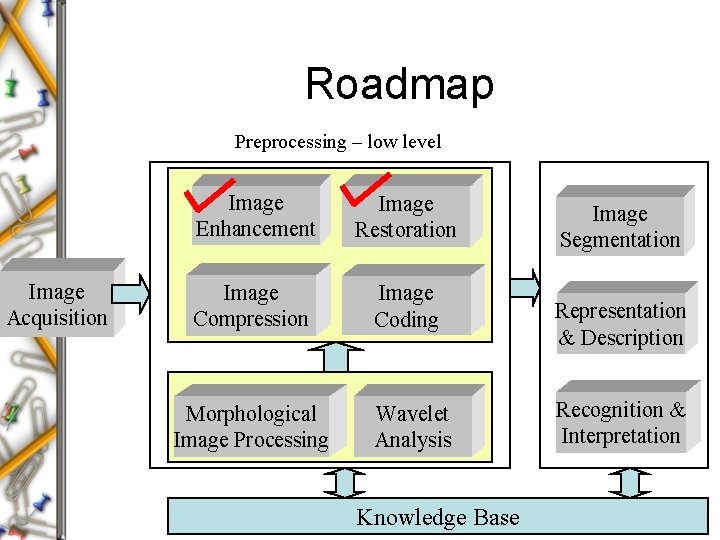
Roadmap Preprocessing – low level Image Acquisition Image Enhancement Image Restoration Image Compression Image Coding Morphological Image Processing Wavelet Analysis Knowledge Base Image Segmentation Representation & Description Recognition & Interpretation

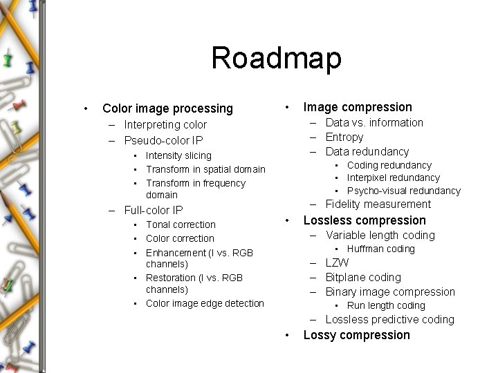
Roadmap • Color image processing • – Data vs. information – Entropy – Data redundancy – Interpreting color – Pseudo-color IP • Intensity slicing • Transform in spatial domain • Transform in frequency domain – Full-color IP • Tonal correction • Color correction • Enhancement (I vs. RGB channels) • Restoration (I vs. RGB channels) • Color image edge detection Image compression • Coding redundancy • Interpixel redundancy • Psycho-visual redundancy – Fidelity measurement • Lossless compression – Variable length coding • Huffman coding – LZW – Bitplane coding – Binary image compression • Run length coding – Lossless predictive coding • Lossy compression

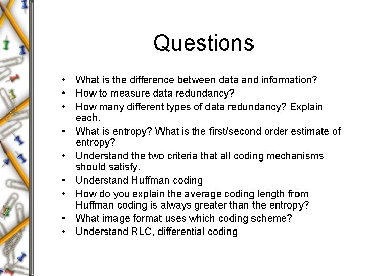
Questions • What is the difference between data and information? • How to measure data redundancy? • How many different types of data redundancy? Explain each. • What is entropy? What is the first/second order estimate of entropy? • Understand the two criteria that all coding mechanisms should satisfy. • Understand Huffman coding • How do you explain the average coding length from Huffman coding is always greater than the entropy? • What image format uses which coding scheme? • Understand RLC, differential coding

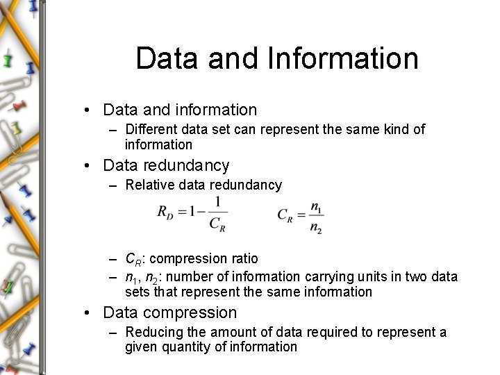
Data and Information • Data and information – Different data set can represent the same kind of information • Data redundancy – Relative data redundancy – CR: compression ratio – n 1, n 2: number of information carrying units in two data sets that represent the same information • Data compression – Reducing the amount of data required to represent a given quantity of information

Data Redundancy • Coding redundancy • Interpixel redundancy • Psychovisual redundancy

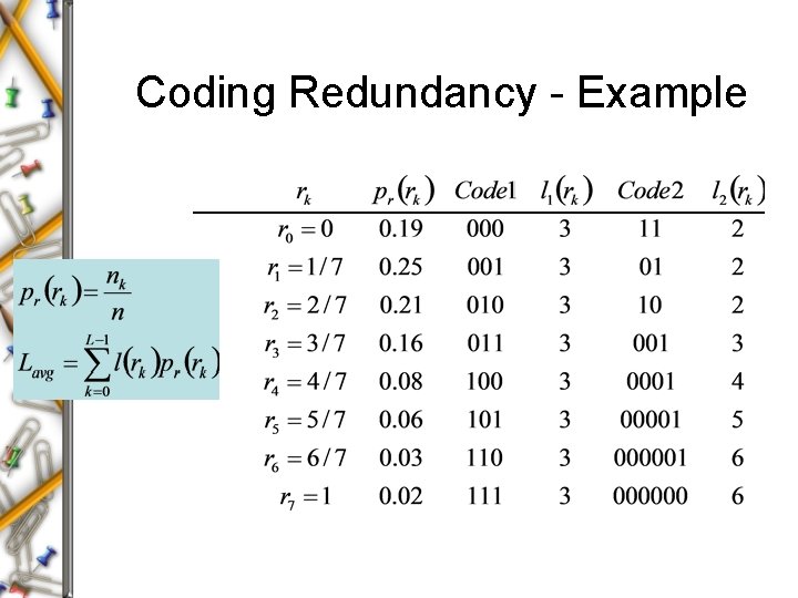
Coding Redundancy • In general, coding redundancy is present when the codes assigned to a set of events (such as gray-level values) have not been selected to take full advantage of the probabilities of the events. • In most images, certain gray levels are more probable than others

Coding Redundancy - Example

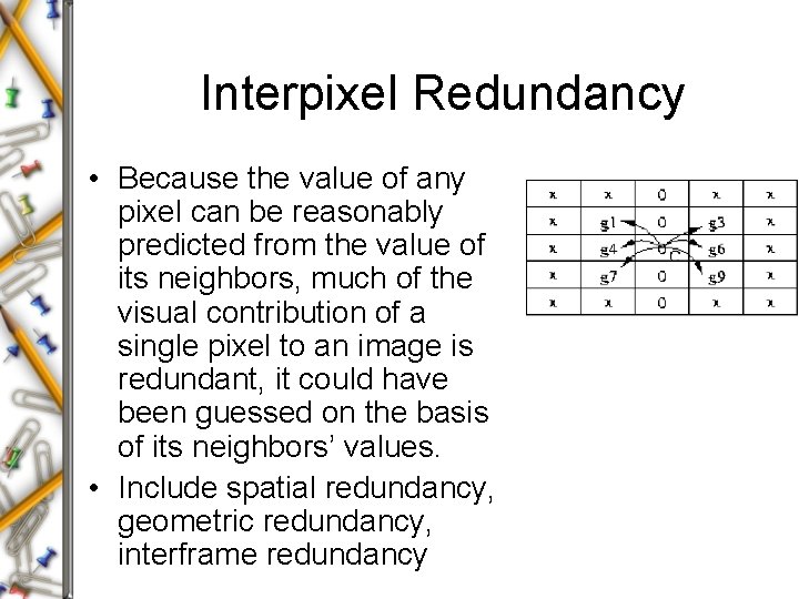
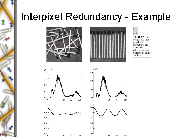
Interpixel Redundancy • Because the value of any pixel can be reasonably predicted from the value of its neighbors, much of the visual contribution of a single pixel to an image is redundant, it could have been guessed on the basis of its neighbors’ values. • Include spatial redundancy, geometric redundancy, interframe redundancy

Interpixel Redundancy - Example

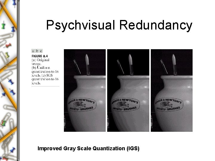
Psychovisual Redundancy • The eye does not respond with equal sensitivity to all visual information. Certain information simply has less relative importance than other information in normal visual processing • In general, an observer searches for distinguishing features such as edges or textural regions and mentally combines them into recognizable groupings.

Psychvisual Redundancy Improved Gray Scale Quantization (IGS)

Evaluation Metrics • Fidelity criteria • Measure information – Entropy

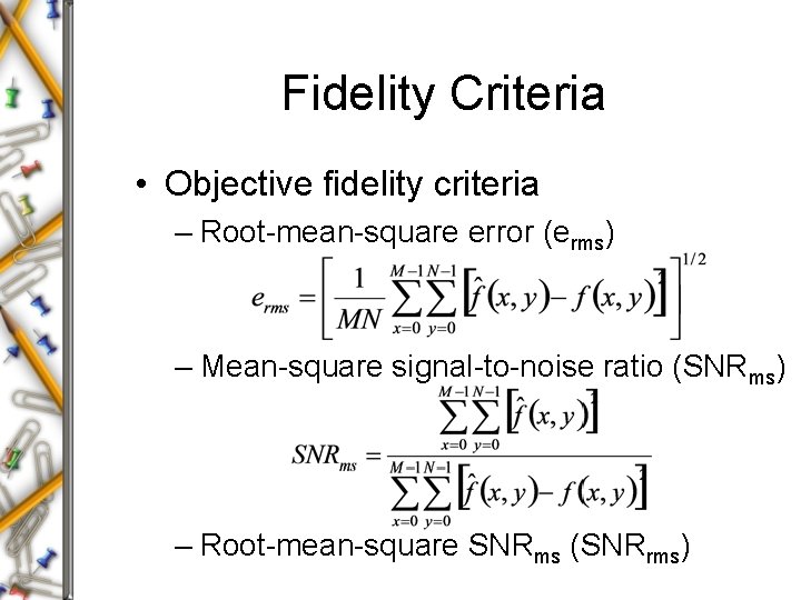
Fidelity Criteria • Objective fidelity criteria – Root-mean-square error (erms) – Mean-square signal-to-noise ratio (SNRms) – Root-mean-square SNRms (SNRrms)

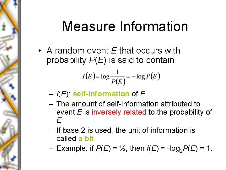
Measure Information • A random event E that occurs with probability P(E) is said to contain – I(E): self-information of E – The amount of self-information attributed to event E is inversely related to the probability of E – If base 2 is used, the unit of information is called a bit – Example: if P(E) = ½, then I(E) = -log 2 P(E) = 1.

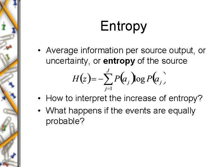
Entropy • Average information per source output, or uncertainty, or entropy of the source • How to interpret the increase of entropy? • What happens if the events are equally probable?

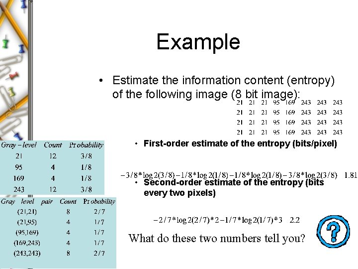
Example • Estimate the information content (entropy) of the following image (8 bit image): • First-order estimate of the entropy (bits/pixel) • Second-order estimate of the entropy (bits every two pixels) What do these two numbers tell you?

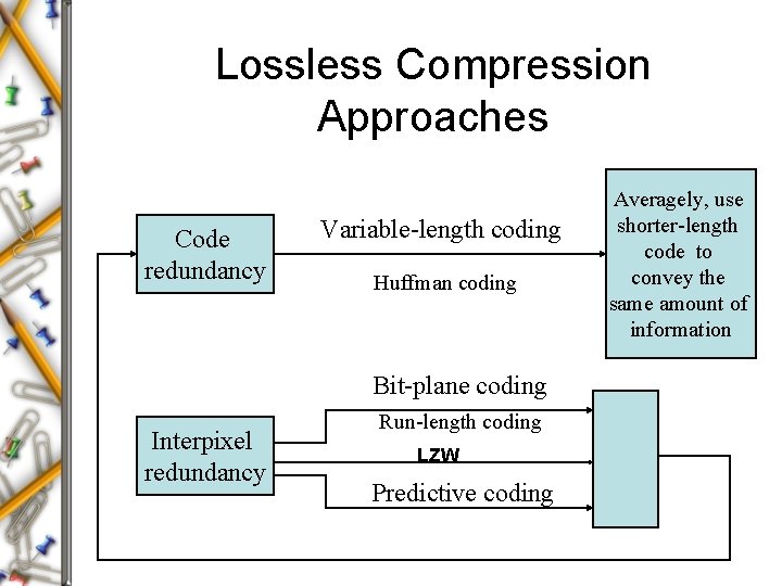
Compression Approaches • Error-free compression or lossless compression – Variable-length coding – Bit-plane coding – Lossless predictive coding • Lossy compression – Lossy predictive coding – Transform coding

Variable-length Coding • Only reduce code redundancy • Assign the shortest possible code words to the most probable gray levels • Huffman coding – Can obtain the optimal coding scheme

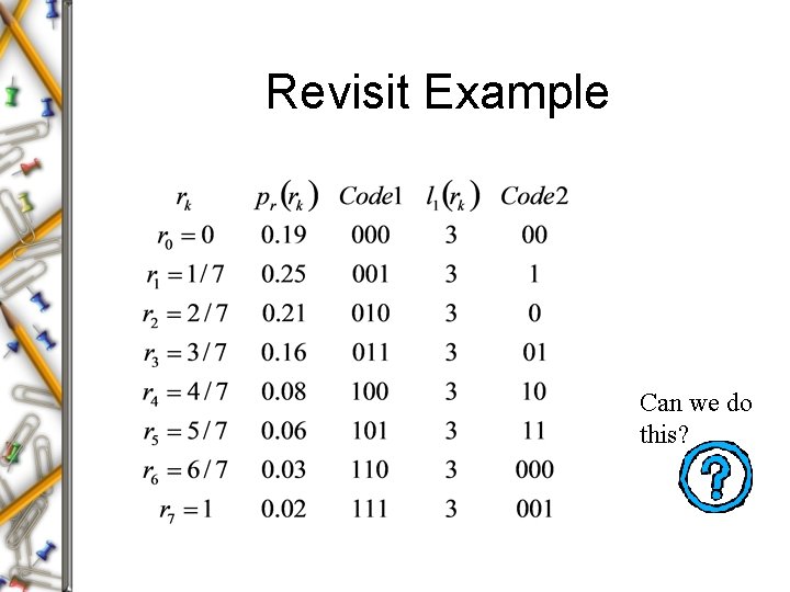
Revisit Example Can we do this?

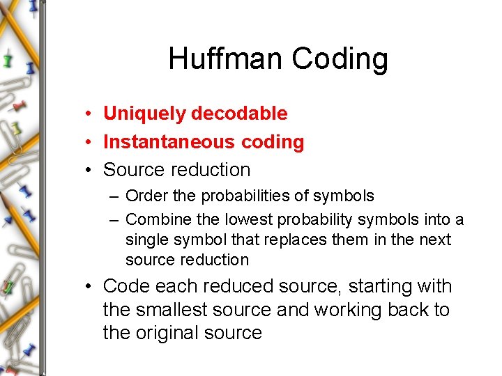
Huffman Coding • Uniquely decodable • Instantaneous coding • Source reduction – Order the probabilities of symbols – Combine the lowest probability symbols into a single symbol that replaces them in the next source reduction • Code each reduced source, starting with the smallest source and working back to the original source

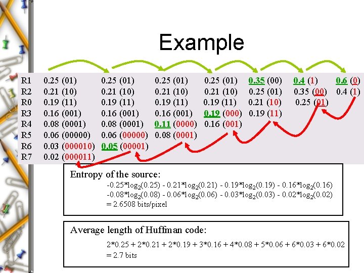
Example R 1 R 2 R 0 R 3 R 4 R 5 R 6 R 7 0. 25 (01) 0. 21 (10) 0. 19 (11) 0. 16 (001) 0. 08 (0001) 0. 06 (00000) 0. 03 (000010) 0. 02 (000011) 0. 25 (01) 0. 21 (10) 0. 19 (11) 0. 16 (001) 0. 08 (0001) 0. 06 (00000) 0. 05 (00001) 0. 25 (01) 0. 21 (10) 0. 19 (11) 0. 16 (001) 0. 11 (0000) 0. 08 (0001) 0. 25 (01) 0. 21 (10) 0. 19 (11) 0. 19 (000) 0. 16 (001) 0. 35 (00) 0. 25 (01) 0. 21 (10) 0. 19 (11) 0. 4 (1) 0. 6 (0) 0. 35 (00) 0. 4 (1) 0. 25 (01) Entropy of the source: -0. 25*log 2(0. 25) - 0. 21*log 2(0. 21) - 0. 19*log 2(0. 19) - 0. 16*log 2(0. 16) -0. 08*log 2(0. 08) - 0. 06*log 2(0. 06) - 0. 03*log 2(0. 03) - 0. 02*log 2(0. 02) = 2. 6508 bits/pixel Average length of Huffman code: 2*0. 25 + 2*0. 21 + 2*0. 19 + 3*0. 16 + 4*0. 08 + 5*0. 06 + 6*0. 03 + 6*0. 02 = 2. 7 bits

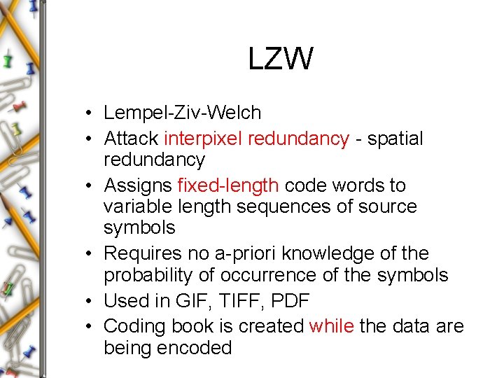
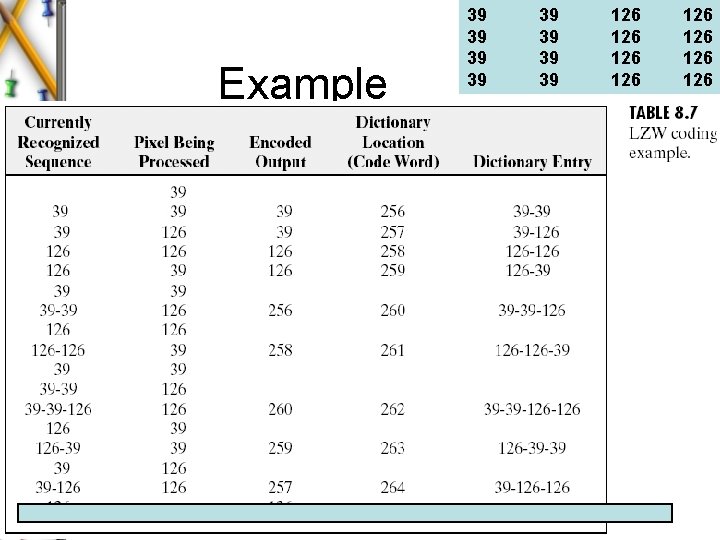
LZW • Lempel-Ziv-Welch • Attack interpixel redundancy - spatial redundancy • Assigns fixed-length code words to variable length sequences of source symbols • Requires no a-priori knowledge of the probability of occurrence of the symbols • Used in GIF, TIFF, PDF • Coding book is created while the data are being encoded

Example 39 39 126 126

Bit-plane Coding • Attack inter-pixel redundancy • First decompose the original image into bit-plane • Binary image compression approach – run-length coding (RLC)

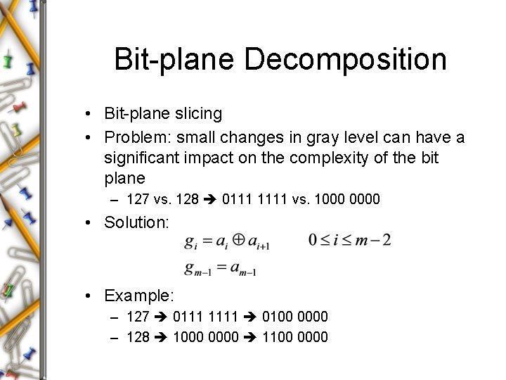
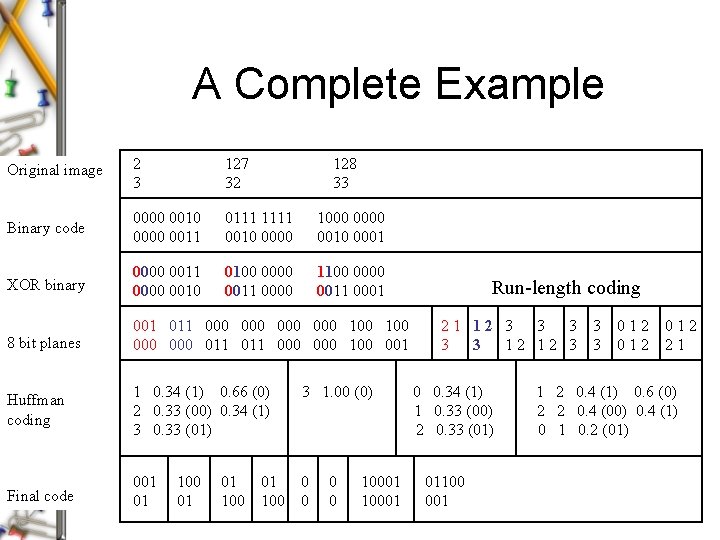
Bit-plane Decomposition • Bit-plane slicing • Problem: small changes in gray level can have a significant impact on the complexity of the bit plane – 127 vs. 128 0111 1111 vs. 1000 0000 • Solution: • Example: – 127 0111 1111 0100 0000 – 128 1000 0000 1100 0000

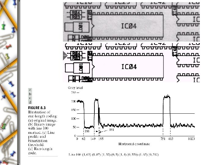
Binary Image Compression RLC • Developed in 1950 s • Standard compression approach in FAX coding • Approach – Code each contiguous group of 0’s or 1’s encountered in a left to right scan of a row by its length – Establish a convention for determining the value of the run – Code black and white run lengths separately using variable-length coding

A Complete Example Original image 2 3 127 32 Binary code 0000 0010 0000 0011 0111 1111 0010 0000 1000 0010 0001 XOR binary 0000 0011 0000 0010 0100 0011 0000 1100 0011 0001 8 bit planes 001 011 000 000 100 000 011 000 100 001 Huffman coding 1 0. 34 (1) 0. 66 (0) 2 0. 33 (00) 0. 34 (1) 3 0. 33 (01) 3 1. 00 (0) Final code 001 01 0 0 100 01 01 100 128 33 01 100 0 0 10001 Run-length coding 21 12 3 3 3 12 12 3 0 0. 34 (1) 1 0. 33 (00) 2 0. 33 (01) 01100 001 3 3 012 012 21 1 2 0. 4 (1) 0. 6 (0) 2 2 0. 4 (00) 0. 4 (1) 0 1 0. 2 (01)

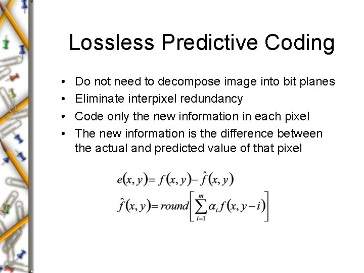
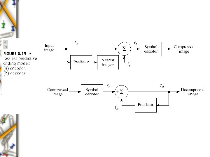
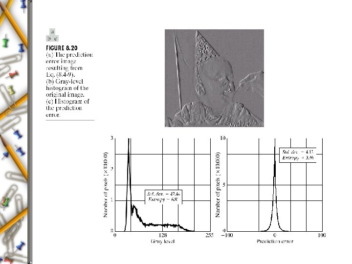
Lossless Predictive Coding • • Do not need to decompose image into bit planes Eliminate interpixel redundancy Code only the new information in each pixel The new information is the difference between the actual and predicted value of that pixel

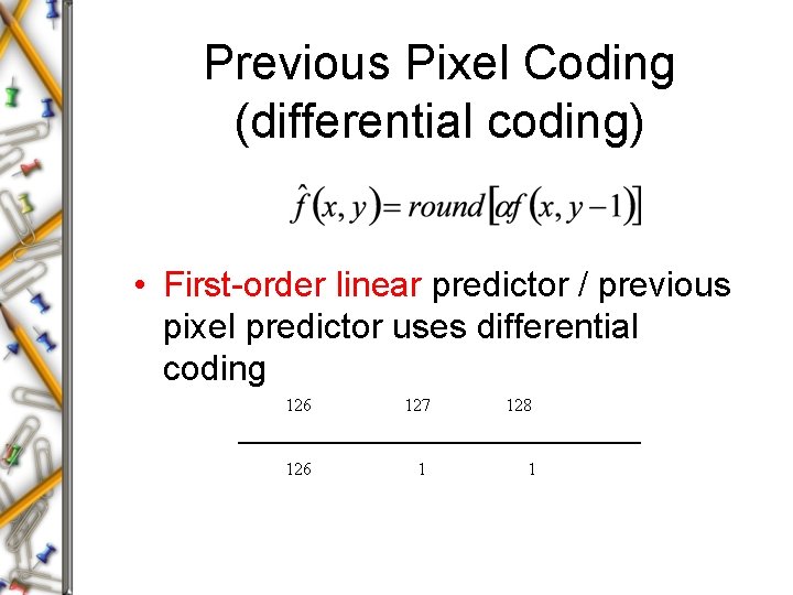
Previous Pixel Coding (differential coding) • First-order linear predictor / previous pixel predictor uses differential coding 126 127 128 126 1 1

Lossless Compression Approaches Code redundancy Variable-length coding Huffman coding Bit-plane coding Interpixel redundancy Run-length coding LZW Predictive coding Averagely, use shorter-length code to convey the same amount of information