DSP C 5000 Chapter 16 Adaptive Filter Implementation

DSP C 5000 Chapter 16 Adaptive Filter Implementation Copyright © 2003 Texas Instruments. All rights reserved.

Outline Adaptive filters and LMS algorithm Implementation of FIR filters on C 54 x Implementation of FIR filters on C 55 x ESIEE, Slide 2

Generalities of Adaptive Filters u u The coefficients of Adaptive filters are variable with time in order to optimize a given criterion. The most commonly used algorithm to adapt the coefficients is the LMS (Least Mean Square) algorithm. Most adaptive filters are implemented as FIR filters, because they are inherently stable. They are widely used in digital communications: w ESIEE, Slide 3 Echo cancellation, equalizers. . .

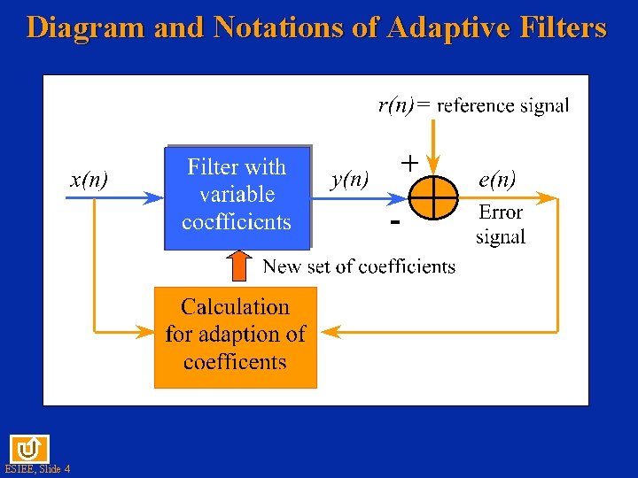
Diagram and Notations of Adaptive Filters ESIEE, Slide 4

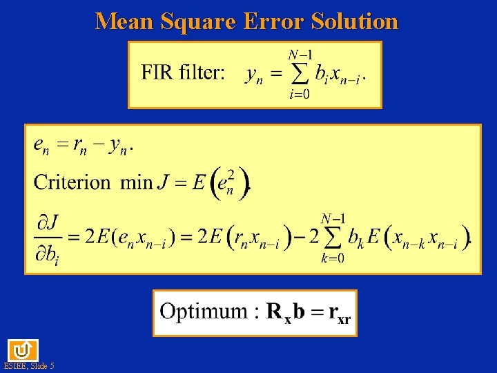
Mean Square Error Solution ESIEE, Slide 5

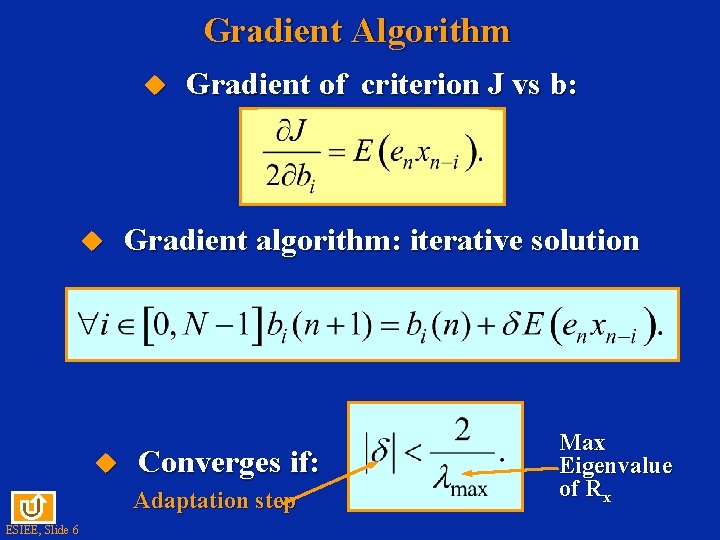
Gradient Algorithm u u u Gradient of criterion J vs b: Gradient algorithm: iterative solution Converges if: Adaptation step ESIEE, Slide 6 Max Eigenvalue of Rx

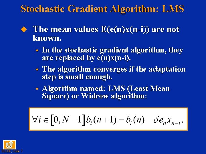
Stochastic Gradient Algorithm: LMS u The mean values E(e(n)x(n-i)) are not known. w w w ESIEE, Slide 7 In the stochastic gradient algorithm, they are replaced by e(n)x(n-i). The algorithm converges if the adaptation step is small enough. Algorithm named: LMS (Least Mean Square) or Widrow algorithm:

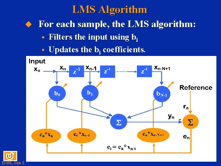
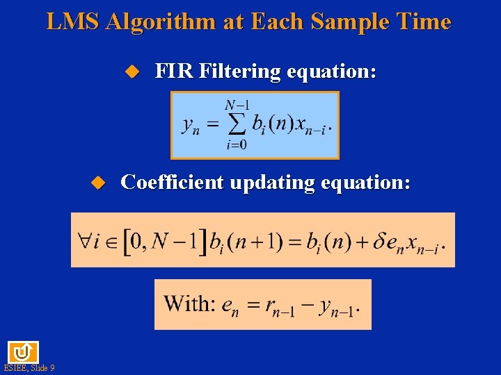
LMS Algorithm u For each sample, the LMS algorithm: w w ESIEE, Slide 8 Filters the input using bi Updates the bi coefficients.

LMS Algorithm at Each Sample Time u u ESIEE, Slide 9 FIR Filtering equation: Coefficient updating equation:

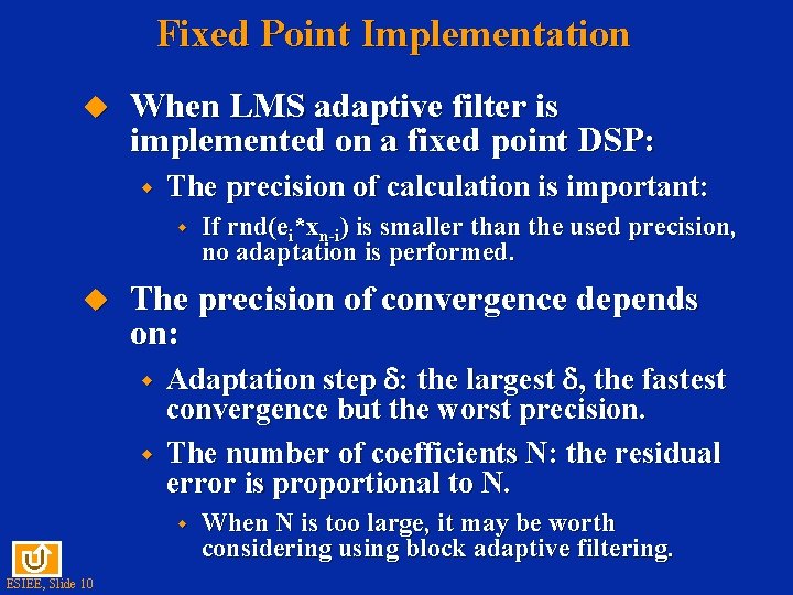
Fixed Point Implementation u When LMS adaptive filter is implemented on a fixed point DSP: w The precision of calculation is important: w u The precision of convergence depends on: w w Adaptation step : the largest , the fastest convergence but the worst precision. The number of coefficients N: the residual error is proportional to N. w ESIEE, Slide 10 If rnd(ei*xn-i) is smaller than the used precision, no adaptation is performed. When N is too large, it may be worth considering using block adaptive filtering.

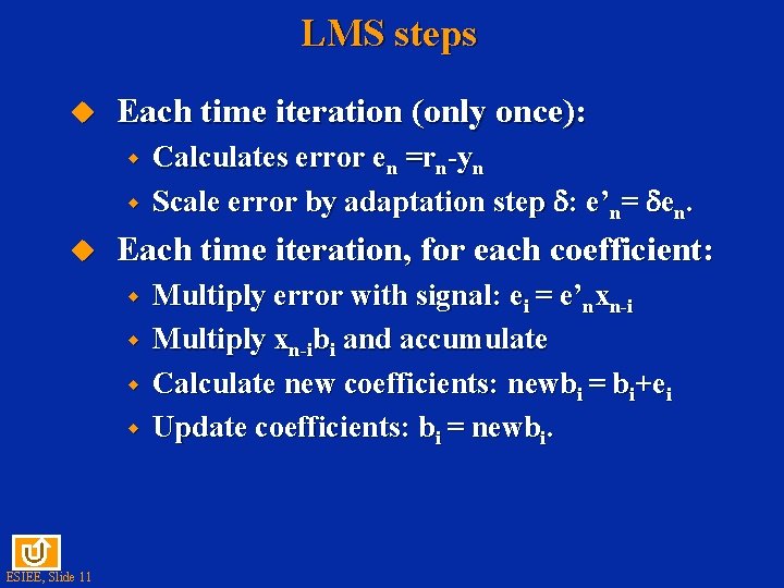
LMS steps u Each time iteration (only once): w w u Each time iteration, for each coefficient: w w ESIEE, Slide 11 Calculates error en =rn-yn Scale error by adaptation step : e’n= en. Multiply error with signal: ei = e’nxn-i Multiply xn-ibi and accumulate Calculate new coefficients: newbi = bi+ei Update coefficients: bi = newbi.

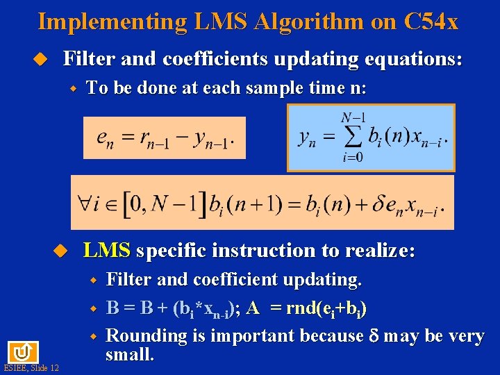
Implementing LMS Algorithm on C 54 x Filter and coefficients updating equations: u w u To be done at each sample time n: LMS specific instruction to realize: w w w ESIEE, Slide 12 Filter and coefficient updating. B = B + (bi*xn-i); A = rnd(ei+bi) Rounding is important because may be very small.

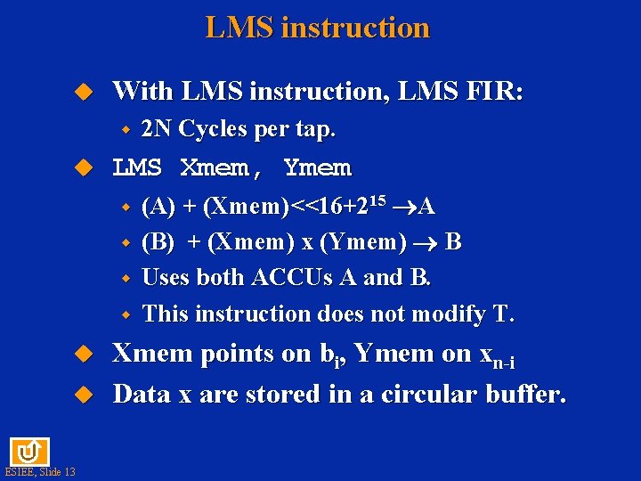
LMS instruction u With LMS instruction, LMS FIR: w u LMS Xmem, Ymem w w u u ESIEE, Slide 13 2 N Cycles per tap. (A) + (Xmem)<<16+215 A (B) + (Xmem) x (Ymem) B Uses both ACCUs A and B. This instruction does not modify T. Xmem points on bi, Ymem on xn-i Data x are stored in a circular buffer.

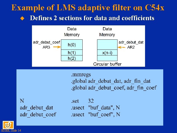
Example of LMS adaptive filter on C 54 x u ESIEE, Slide 14 Defines 2 sections for data and coefficients

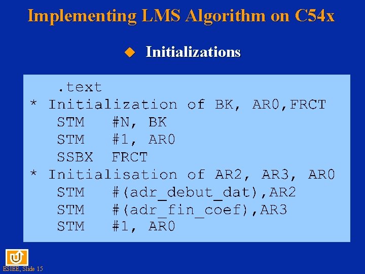
Implementing LMS Algorithm on C 54 x u ESIEE, Slide 15 Initializations

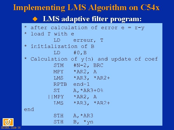
Implementing LMS Algorithm on C 54 x u ESIEE, Slide 16 LMS adaptive filter program:

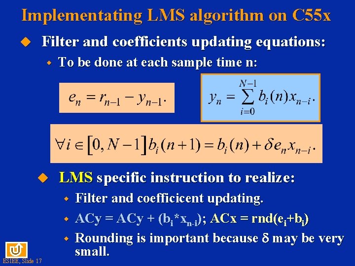
Implementating LMS algorithm on C 55 x u Filter and coefficients updating equations: w u To be done at each sample time n: LMS specific instruction to realize: w w w ESIEE, Slide 17 Filter and coefficicent updating. ACy = ACy + (bi*xn-i); ACx = rnd(ei+bi) Rounding is important because may be very small.

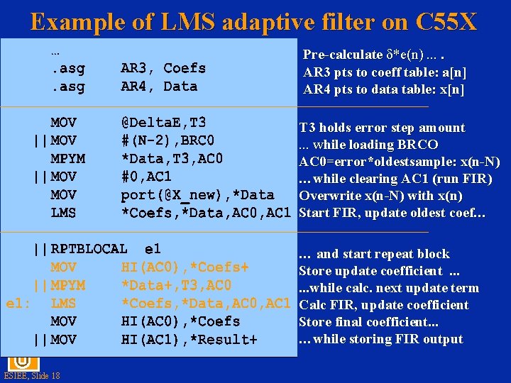
Example of LMS adaptive filter on C 55 X Pre-calculate *e(n). . AR 3 pts to coeff table: a[n] AR 4 pts to data table: x[n] T 3 holds error step amount. . . while loading BRCO AC 0=error*oldestsample: x(n-N) …while clearing AC 1 (run FIR) Overwrite x(n-N) with x(n) Start FIR, update oldest coef… … and start repeat block Store update coefficient. . . while calc. next update term Calc FIR, update coefficient Store final coefficient. . . …while storing FIR output ESIEE, Slide 18

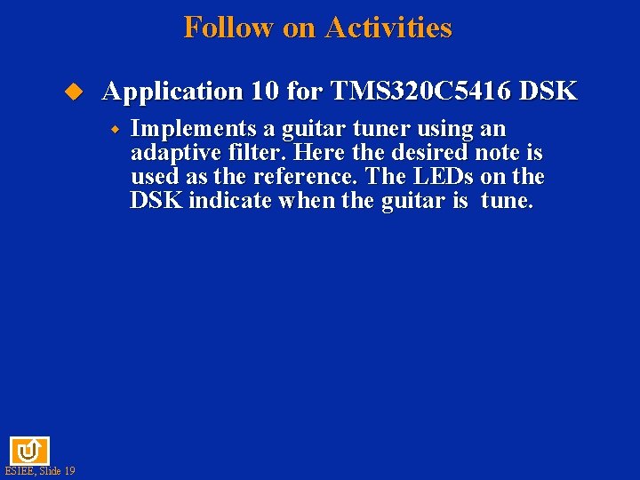
Follow on Activities u Application 10 for TMS 320 C 5416 DSK w ESIEE, Slide 19 Implements a guitar tuner using an adaptive filter. Here the desired note is used as the reference. The LEDs on the DSK indicate when the guitar is tune.