DiscreteTime Signal Processing DSP ChuSong Chen Email songiis

Discrete-Time Signal Processing (DSP) Chu-Song Chen Email: song@iis. sinica. du. tw Institute of Information Science, Academia Sinica Institute of Networking and Multimedia, National Taiwan University Fall 2006

What are Signals (c. f. Kuhn 2005 and Oppenheim et al. 1999) flow of information: generally convey information about the state or behavior of a physical system. Ø measured quantity that varies with time (or position) Ø electrical signal received from a transducer (microphone, thermometer, accelerometer, antenna, etc. ) Ø electrical signal that controls a process continuous-time signal: Also know as analog signal. Ø voltage, current, temperature, speed, speech signal, etc. discrete-time signal: daily stock market price, daily average temperature, sampled continuous signals.

Examples of Signals types in dimensionality: Ø speech signal: represented as a function over time. -- 1 D signal Ø image signal: represented as a brightness function of two spatial variables. -- 2 D signal Ø ultra sound data or image sequence – 3 D signal Electronics can only deal easily with time-dependent signals, therefore spatial signals, such as images, are typically first converted into a time signal with a scanning process (TV, fax, etc. )

Generation of Discrete-time Signal In practice, discrete-time signal can often arise from periodic sampling of an analog signal.

What is Signal Processing (Kuhn 2005) Signals may have to be transformed in order to Ø amplify or filter out embedded information Ø detect patterns Ø prepare the signal to survive a transmission channel Ø undo distortions contributed by a transmission channel Ø compensate for sensor deficiencies Ø find information encoded in a different domain. To do so, we also need: Ø methods to measure, characterize, model, and simulate signals. Ø mathematical tools that split common channels and transformations into easily manipulated building blocks.

Analog Electronics for Signal Processing (Kuhn 2005) Passive networks (resistors, capacities, inductivities, crystals, nonlinear elements: diodes …), (roughly) linear operational amplifiers Advantages: Ø passive networks are highly linear over a very large dynamic range and bandwidths. Ø analog signal-processing circuits require little or no power. Ø analog circuits cause little additional interference

Digital Signal Processing (Kuhn 2005) Analog/digital and digital/analog converters, CPU, DSP, ASIC, FPGA Advantages: Ø noise is easy to control after initial quantization Ø highly linear (with limited dynamic range) Ø complex algorithms fit into a single chip Ø flexibility, parameters can be varied in software Ø digital processing in insensitive to component tolerances, aging, environmental conditions, electromagnetic inference But Ø discrete time processing artifacts (aliasing, delay) Ø can require significantly more power (battery, cooling) Ø digital clock and switching cause interference

Typical DSP Applications (Kuhn 2005) Ø communication systems modulation/demodulation, channel equalization, echo cancellation Ø consumer electronics perceptual coding of audio and video on DVDs, speech synthesis, speech recognition Ø Music synthetic instruments, audio effects, noise reduction Ø medical diagnostics Magnetic-resonance and ultrasonic imaging, computer tomography, ECG, EEG, MEG, AED, audiology Ø Geophysics seismology, oil exploration Ø astronomy VLBI, speckle interferometry Ø experimental physics sensor data evaluation Ø aviation radar, radio navigation Ø security steganography, digital watermarking, biometric identification, visual surveillance systems, signal intelligence, electronic warfare Ø engineering control systems, feature extraction for pattern recognition

Syllabus (c. f. Kuhn 2005 and Stearns 2002) Ø Signals and systems: Discrete sequences and systems, their types and properties. Linear time-invariant systems, correlation/convolution, eigen functions of linear time-invariant systems. Review of complex arithmetics. Ø Fourier transform: Harmonic analysis as orthogonal base functions. Forms of the Fourier transform. Convolution theorem. Dirac’s delta function. Impulse trains (combs) in the time and frequency domain. Ø Discrete sequences and spectra: Periodic sampling of continuous signals, periodic signals, aliasing, sampling and reconstruction of lowpass signals. Ø Discrete Fourier transform: continuous versus discrete Fourier transform, symmetric, linearity, fast Fourier transform (FFT). Ø Spectral estimation: power spectrum. Ø Finite and infinite impulse-response filters: Properties of filters, implementation forms, window-based FIR design, use of analog IIR techniques (Butterworth, Chebyshev I/II, etc. )

Ø Z-transform: zeros and poles, difference equations, direct form I and II. Ø Random sequences and noise: Random variables, stationary process, auto-correlation, cross-correlation, deterministic cross-correlation sequences, white noise. Ø Multi-rate signal processing: decimation, interpolation, polyphase decompositions. Ø Adaptive signal processing: mean-squared performance surface, LMS algorithm, Direct descent and the RLS algorithm. Ø Coding and Compression: Transform coding, discrete cosine transform, multirate signal decomposition and subband coding, PCA and KL transformation. Ø Wavelet transform: Time-frequency analysis. Discrete wavelet transform (DFT), DFT for compression. Ø Particle filtering: hidden Markov model, state space form, Markov chain Monte Carlo (MCMC), unscented Kalman filtering, particle filtering for tracking.

Lectures: 12 times. References: Ø S. D. Stearns, Digital Signal Processing with Examples in MATLAB, CRC Press, 2003. (main textbook, but not dominant) Ø B. A. Shenoi, Introduction to Signal Processing and Filter Design, Wiley, 2006. Ø S. Salivahanan, A. Vallavaraj, and C. Gnanapriya, Digital Signal Procesing, Mc. Graw-Hill, 2002. Ø A. V. Oppenheim and R. W. Schafer, Discrete Time Signal Processing, 2 nd ed. , Prentice Hall, 1999. Ø J. H. Mc. Clellan, R. W. Schafer, and M. A. Yoder, Signal Processing First, Prentice Hall, 2004. (suitable for beginners) Ø S. K. Mitra, Digital Signal Processing, A Computer-Based Approach, Mc. Graw-Hill, 2002. Ø Markus Kuhn, Digital Signal Processing slides in Cambridge, http: //www. c 1. cam. ac. uk/Teaching/2005/DSP Ø Some relevant papers …

Main journals and conferences in this field Journal Ø IEEE Transactions on Signal Processing Ø EUROSIP Journal on Applied Signal Processing Ø… Conference Ø IEEE ICASSP (International Conference on Acoustics, Speech, and Signal Processing) Evaluations in this course Homework – about three times. Tests: twice Term project

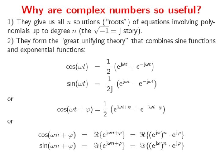
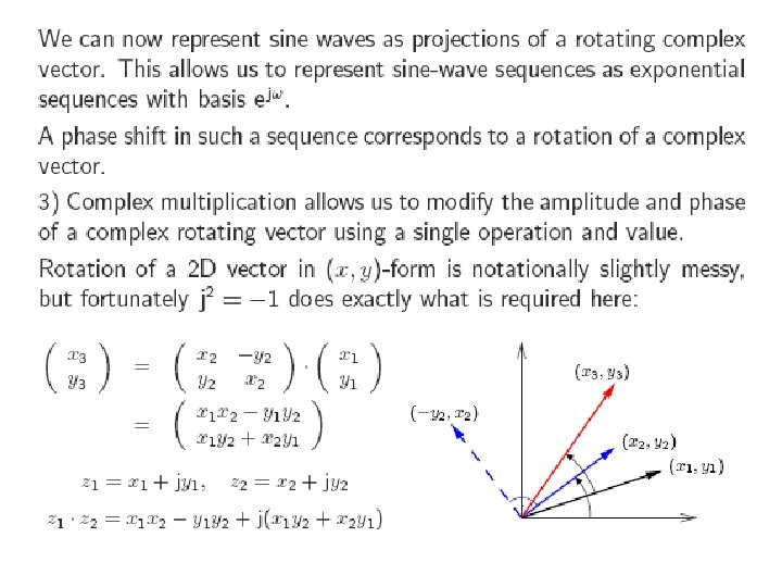
Review of complex exponential (c. f. Kuhn 2005 and Oppenheim et al. 1999) geometric series is used repeatedly to simplify expressions in DSP. Ø if the magnitude of x is less than one, then In DSP, the geometric series is often a complex exponential variable of the form ejk, where j =

For example (1)

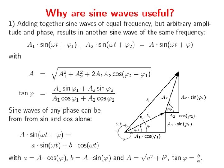
Trigonometric Identities

Trigonometric functions, especially sine and cosine functions, appear in different combinations in all kinds of harmonic analysis: Fourier series, Fourier transforms, etc. Advantages of complex exponential The identities that give sine and cosine functions in terms of exponentials are important – because they allow us to find sums of sines and cosines using the geometric series. Eg. from (1), we have ie. a sum of equally spaced samples of any sine or cosine function is zero, provided the sum is over a cycle (or a number of cycles), of the function.

Least Squares and Orthogonality (c. f. Stearns, 2003, Chap. 2) least squares: Suppose we have two continuous functions, f(t) and g(c, t), where c is a parameter (or a set of parameters). If c is selected to minimize the total squared error (TSE) assume

An example of continuous least-squares approximation

In DSP, least squares approximations are made more often to discrete (sampled) data, rather than to continuous data

If the approximating function is again g(c, t), the total squared error in the discrete case is now given as where fn is the nth element of f, and T is the time step (interval between samples). Assume that there are M basis functions (or bases), g 1, …, g. M, to represent g. TSE =

Let us denote that (where ’ means matrix transpose)

This is represented in MATLAB form, where x = Ab means that x is the solution of the linear equation system Ax = b. In this case, c = (GTG)-1 GTb, when GTG is nonsingular.

Matrix derivation: Least squares can be derived via another way by using matrix derivations: TSE = Let b = f. T = [f 1, …, fn]T, then TSE = ||b – Gc||2 = (b – Gc)T(b – Gc). When GTG is nonsingular,

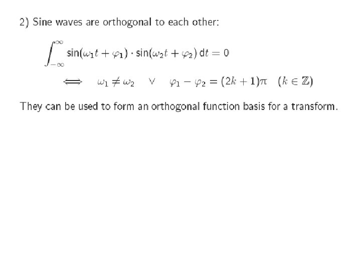
Orthogonal bases (or orthogonal basis functions): In many cases, we hope the bases to be ‘orthogonal’ to each other. (if two row vectors a and b are orthogonal, then the inner product ab’ = 0) Advantage: suppose the n functions are mutually orthogonal with respect to the N samples, then each equation in solving the least squares becomes the solution of c becomes very simple:

An intuitive explanation: orthographic projection The solution of c is the “orthographic projection” of the input vector f onto the subspace formed by the orthogonal bases. We can change the number of bases, M, and the solution still remains as the same form. Ø Choosing the number of bases to represent a signal establish the fundamental concept of signal compression.

Discrete Fourier Series (c. f. Stearns, 2003, Chap. 2) Harmonic analysis: A discrete Foruier series consisits of combinations of sampled sine and cosine functions. It forms the basis of a branch of mathematics called harmonic analysis, which is applicable to the study of all kinds of natural phenomena, including the motion of stars and planets and atoms, acoustic waves, radio waves, etc. Let x = [x 1, …, x. N-1]. If we say the fundamental period of x is N samples, we image that the samples of x repeat, over and over again, in the time domain.

Sample vector and periodic extension; N=50

The fundamental period is N samples, or NT seconds, where T is the time step in seconds. The fundamental frequency is the reciprocal of the fundamental period, f 0 = 1/NT Hertz (HZ). ‘Hertz’ means “cycles per second. ” Another unit of frequency besides f is rad/s (radians per second)

Fourier Series (a least-square approximation using sine and cosine bases)

Equivalence of Fourier Series Coefficients

If the fundamental period 2 /w 0 covers N samples or NT seconds, then the fundamental frequency must be With this substitution to indicate sampling over exactly one fundamental period:

In this form, the harmonic functions are orthogonal with respect to the N samples of x: These results can be proved by using the trigonometric identities and the geometric series application. Ø We can use least squares principle to determine the best coefficients am and bm.

By applying the orthographic projection, the least-squares Fourier coefficients are When we use the complex exponential as bases, the coefficients cm can be determined by am and bm as: ’ means the complex conjugate.

or equivalently The results also suggest a continuous form of the Fourier series. We can image decreasing the time step, T, toward zero, and at the same time increasing N in a way such that the period, NT, remains constant. Thje samples (xn) or x(t) are thus packed more densely, so that, in the limit, we have the Fourier series for a continuous periodic function:

Sometimes, for the sake of symmetry, cm is given by an integral around t=0: The continuous forms of the Fourier series are, nevertheless, applicable to a wide range of natural periodic phenomena. We have introduced two forms of the discrete Fourier series, and show to calculate the coefficients when the samples are taken over one fundamental period of the data.