Diploma Macro Paper 2 Monetary Macroeconomics Lecture 6

Diploma Macro Paper 2 Monetary Macroeconomics Lecture 6 Aggregate supply and putting AD and AS together Mark Hayes 1

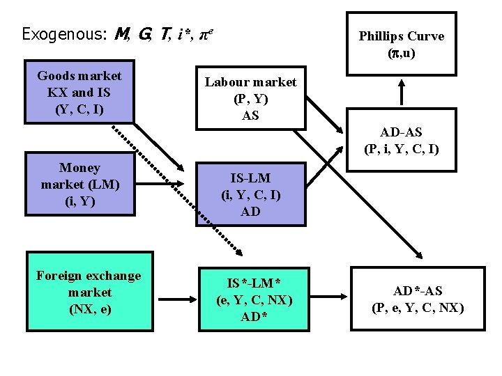
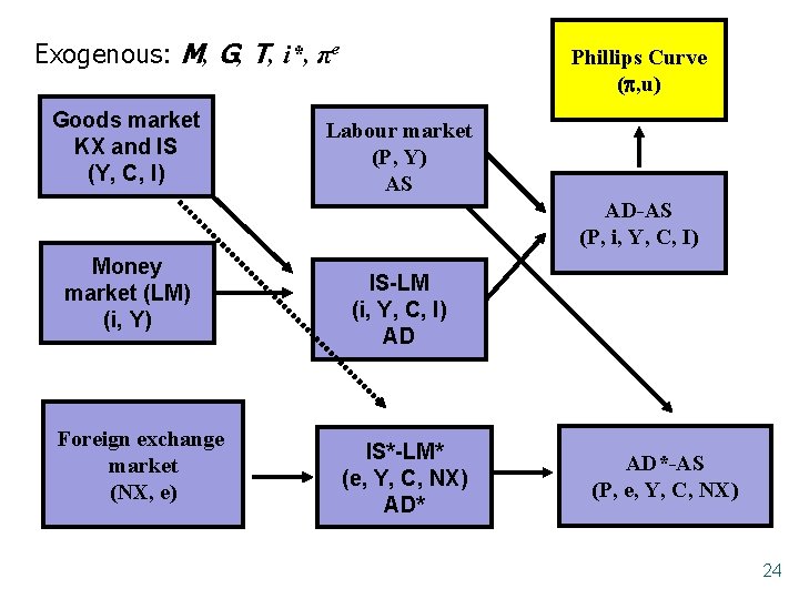
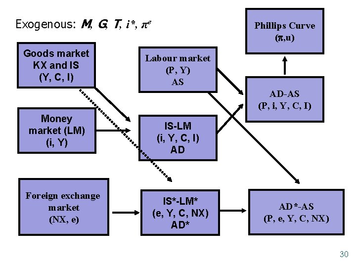
Exogenous: M, G, T, i*, πe Goods market KX and IS (Y, C, I) Phillips Curve ( , u) Labour market (P, Y) AS AD-AS (P, i, Y, C, I) Money market (LM) (i, Y) Foreign exchange market (NX, e) IS-LM (i, Y, C, I) AD IS*-LM* (e, Y, C, NX) AD*-AS (P, e, Y, C, NX)

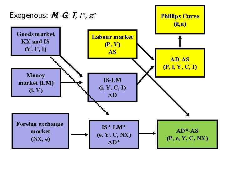
Exogenous: M, G, T, i*, πe Goods market KX and IS (Y, C, I) Phillips Curve ( , u) Labour market (P, Y) AS AD-AS (P, i, Y, C, I) Money market (LM) (i, Y) Foreign exchange market (NX, e) IS-LM (i, Y, C, I) AD IS*-LM* (e, Y, C, NX) AD*-AS (P, e, Y, C, NX)

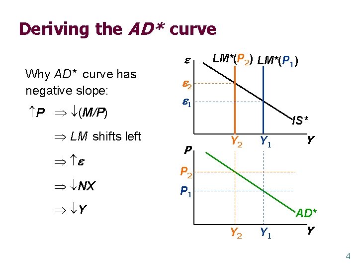
Deriving the AD* curve Why AD* curve has negative slope: P (M/P) LM shifts left NX LM*(P 2) LM*(P 1) 2 1 IS* P Y 2 Y 1 Y P 2 P 1 Y AD* Y 2 Y 1 Y 4

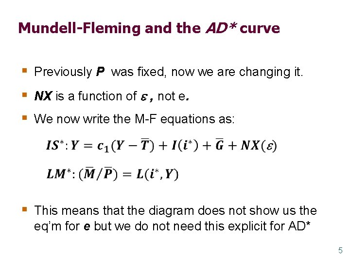
Mundell-Fleming and the AD* curve § Previously P was fixed, now we are changing it. § NX is a function of , not e. § We now write the M-F equations as: § This means that the diagram does not show us the eq’m for e but we do not need this explicit for AD* 5

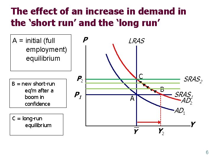
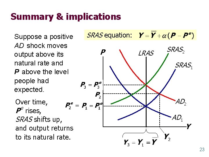
The effect of an increase in demand in the ‘short run’ and the ‘long run’ P A = initial (full employment) equilibrium B = new short-run eq’m after a boom in confidence C = long-run equilibrium LRAS C P 2 P 1 SRAS 2 B A Y 2 SRAS 1 AD 2 AD 1 Y 6

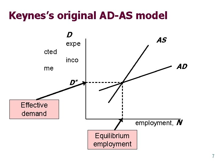
Keynes’s original AD-AS model D AS expe cted inco AD me D* Effective demand employment, N Equilibrium employment 7

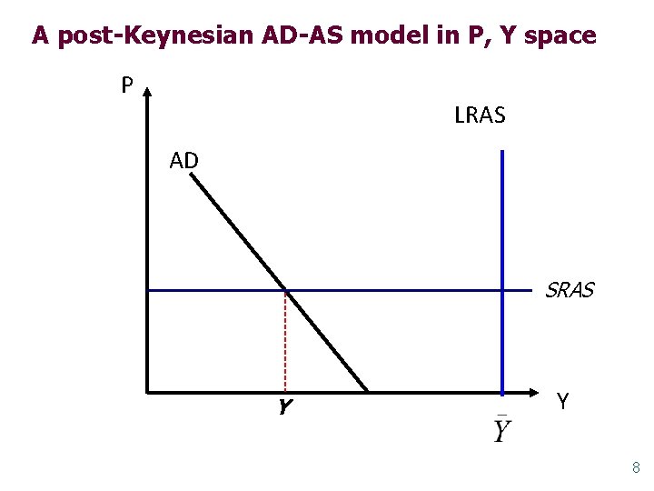
A post-Keynesian AD-AS model in P, Y space P LRAS AD SRAS Y Y 8

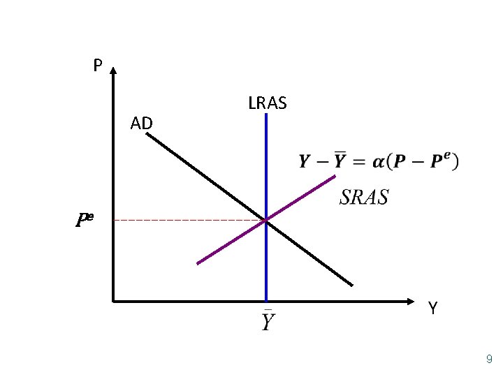
P AD LRAS Pe Y 9

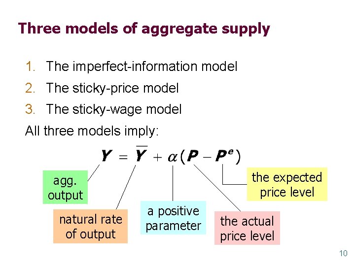
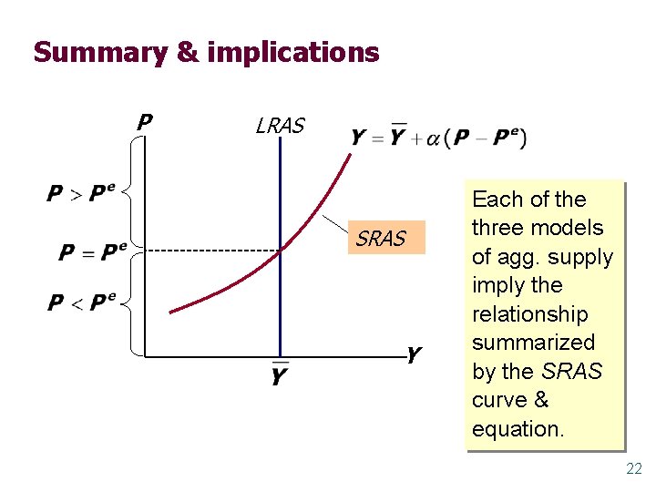
Three models of aggregate supply 1. The imperfect-information model 2. The sticky-price model 3. The sticky-wage model All three models imply: the expected price level agg. output natural rate of output a positive parameter the actual price level 10

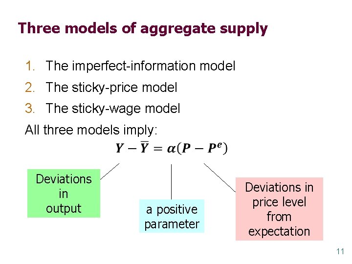
Three models of aggregate supply 1. The imperfect-information model 2. The sticky-price model 3. The sticky-wage model All three models imply: Deviations in output a positive parameter Deviations in price level from expectation 11

The imperfect-information model Assumptions: § All wages and prices are perfectly flexible, all markets clear § Each supplier produces one good, consumes many goods. § Supply of each good depends on its relative price: the nominal price of the good divided by the overall price level. 12

The imperfect-information model § All suppliers know the nominal price of the good they produce, but do not know the general price level. § Supplier does not know general price level at the time of the production decision, so uses the expected price level, P e. § Suppose P rises but P e does not. § Supplier thinks it is their own relative price which § has risen, so produces more. With many producers thinking this way, e Y will rise whenever P rises above P. 13

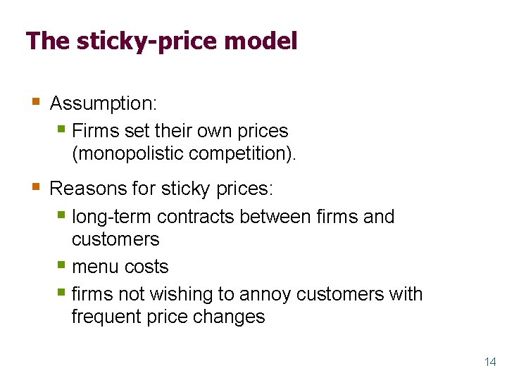
The sticky-price model § Assumption: § Firms set their own prices (monopolistic competition). § Reasons for sticky prices: § long-term contracts between firms and customers § menu costs § firms not wishing to annoy customers with frequent price changes 14

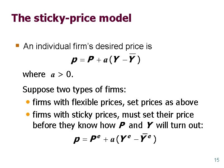
The sticky-price model § An individual firm’s desired price is where a > 0. Suppose two types of firms: • firms with flexible prices, set prices as above • firms with sticky prices, must set their price before they know how P and Y will turn out: 15

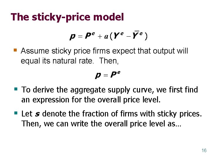
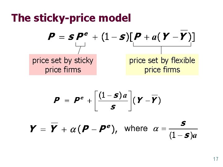
The sticky-price model § Assume sticky price firms expect that output will equal its natural rate. Then, § To derive the aggregate supply curve, we first find an expression for the overall price level. § Let s denote the fraction of firms with sticky prices. Then, we can write the overall price level as… 16

The sticky-price model price set by sticky price firms price set by flexible price firms 17

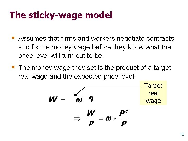
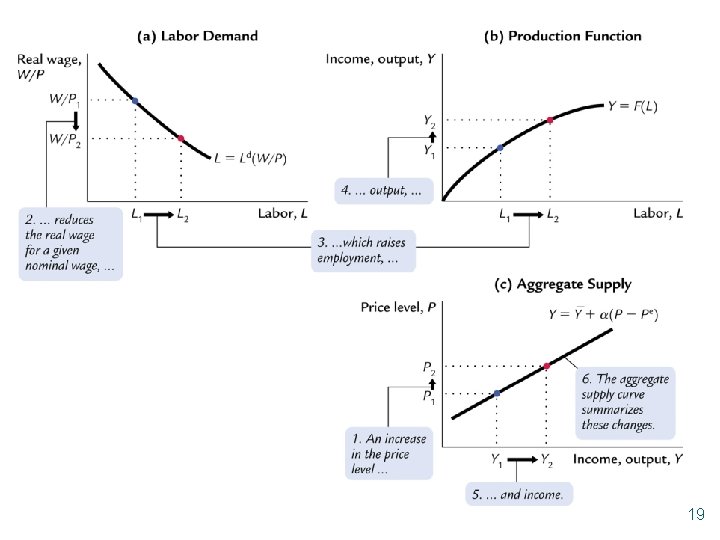
The sticky-wage model § Assumes that firms and workers negotiate contracts and fix the money wage before they know what the price level will turn out to be. § The money wage they set is the product of a target real wage and the expected price level: Target real wage 18

19

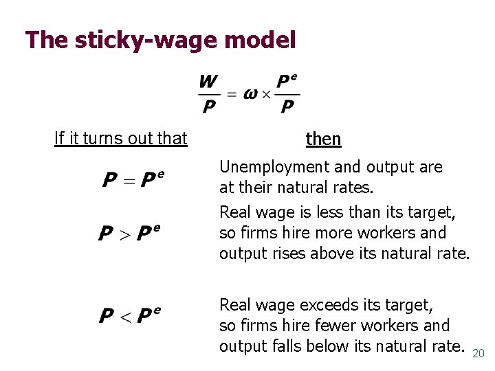
The sticky-wage model If it turns out that then Unemployment and output are at their natural rates. Real wage is less than its target, so firms hire more workers and output rises above its natural rate. Real wage exceeds its target, so firms hire fewer workers and output falls below its natural rate. 20

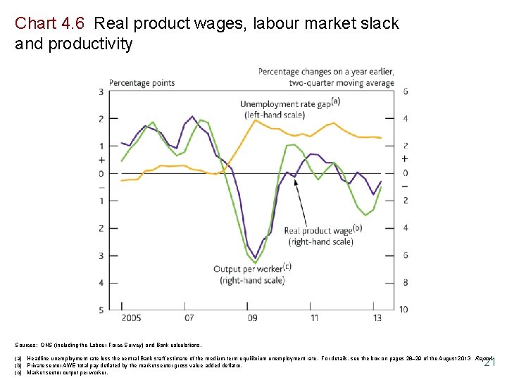
Chart 4. 6 Real product wages, labour market slack and productivity Sources: ONS (including the Labour Force Survey) and Bank calculations. (a) Headline unemployment rate less the central Bank staff estimate of the medium-term equilibrium unemployment rate. For details, see the box on pages 28– 29 of the August 2013 Report. (b) Private sector AWE total pay deflated by the market sector gross value added deflator. (c) Market sector output per worker. 21

Summary & implications P LRAS SRAS Y Each of the three models of agg. supply imply the relationship summarized by the SRAS curve & equation. 22

Summary & implications Suppose a positive AD shock moves output above its natural rate and P above the level people had expected. Over time, P e rises, SRAS shifts up, and output returns to its natural rate. SRAS equation: P LRAS SRAS 2 SRAS 1 AD 2 AD 1 Y 23

Exogenous: M, G, T, i*, πe Goods market KX and IS (Y, C, I) Phillips Curve ( , u) Labour market (P, Y) AS AD-AS (P, i, Y, C, I) Money market (LM) (i, Y) Foreign exchange market (NX, e) IS-LM (i, Y, C, I) AD IS*-LM* (e, Y, C, NX) AD*-AS (P, e, Y, C, NX) 24

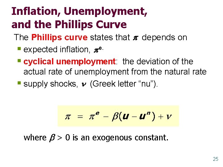
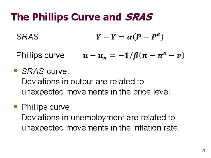
Inflation, Unemployment, and the Phillips Curve The Phillips curve states that depends on § expected inflation, e. § cyclical unemployment: the deviation of the actual rate of unemployment from the natural rate § supply shocks, (Greek letter “nu”). where > 0 is an exogenous constant. 25

The Phillips Curve and SRAS Phillips curve § SRAS curve: Deviations in output are related to unexpected movements in the price level. § Phillips curve: Deviations in unemployment are related to unexpected movements in the inflation rate. 26

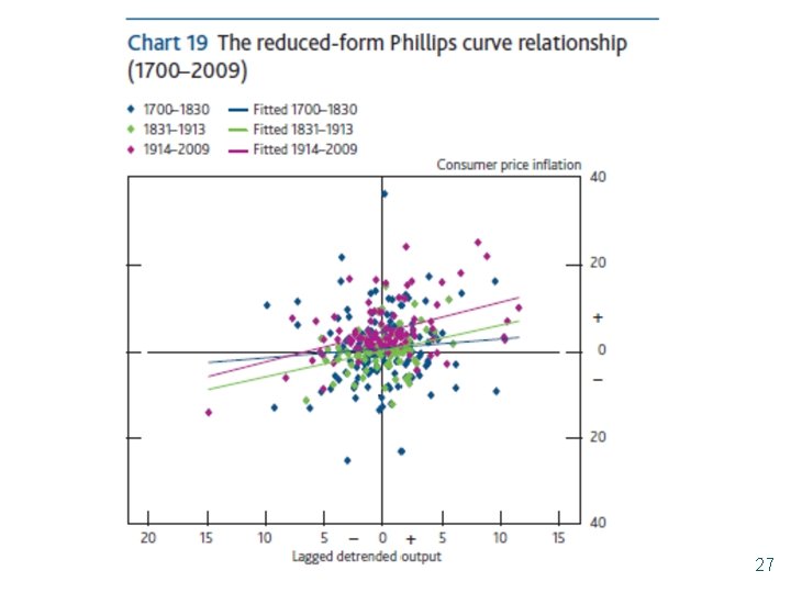
27

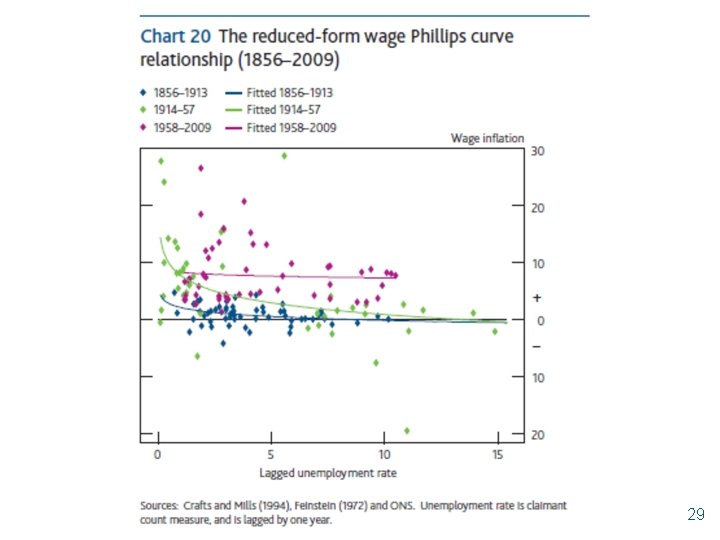
28

29

Exogenous: M, G, T, i*, πe Goods market KX and IS (Y, C, I) Phillips Curve ( , u) Labour market (P, Y) AS AD-AS (P, i, Y, C, I) Money market (LM) (i, Y) Foreign exchange market (NX, e) IS-LM (i, Y, C, I) AD IS*-LM* (e, Y, C, NX) AD*-AS (P, e, Y, C, NX) 30

Next term § Policy effectiveness and inflation targeting § Origins of the North Atlantic and Euro crises 31