Diploma Macro Paper 2 Monetary Macroeconomics Lecture 4

Diploma Macro Paper 2 Monetary Macroeconomics Lecture 4 Aggregate demand: Using IS-LM to understand fiscal and monetary policy Mark Hayes slide 1

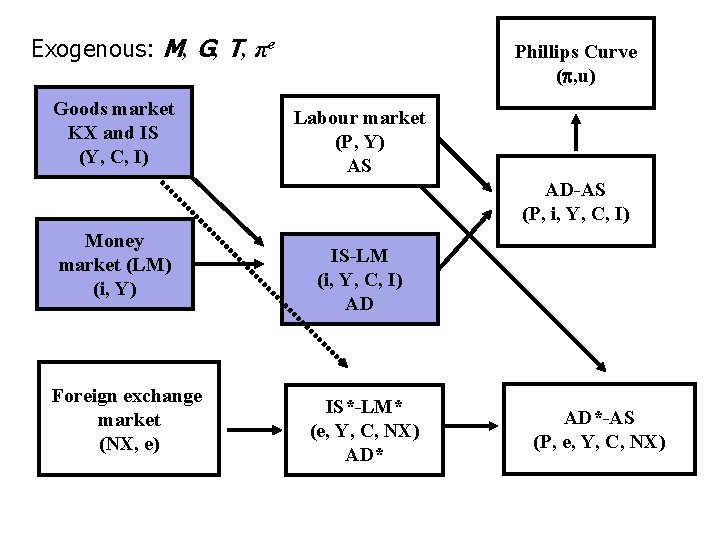
Exogenous: M, G, T, πe Goods market KX and IS (Y, C, I) Phillips Curve ( , u) Labour market (P, Y) AS AD-AS (P, i, Y, C, I) Money market (LM) (i, Y) Foreign exchange market (NX, e) IS-LM (i, Y, C, I) AD IS*-LM* (e, Y, C, NX) AD*-AS (P, e, Y, C, NX)

Outline § Applying the IS-LM model: – Fiscal policy – Monetary policy – Interaction between them § UK experience since 2008 slide 3

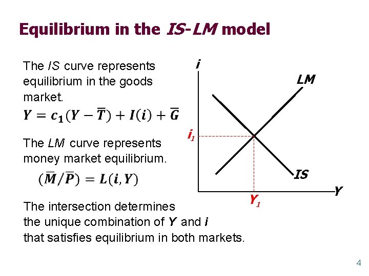
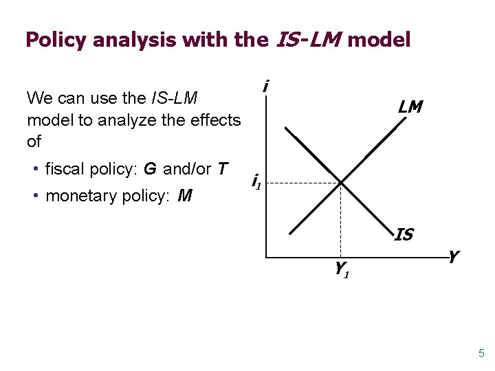
Equilibrium in the IS -LM model The IS curve represents equilibrium in the goods market. i LM The LM curve represents money market equilibrium. i 1 IS The intersection determines the unique combination of Y and i that satisfies equilibrium in both markets. Y 1 Y 4

Policy analysis with the IS -LM model We can use the IS-LM model to analyze the effects of • fiscal policy: G and/or T • monetary policy: M i LM i 1 IS Y 1 Y 5

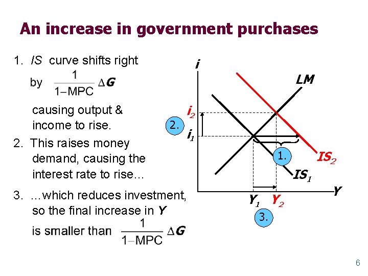
An increase in government purchases 1. IS curve shifts right causing output & income to rise. 2. This raises money demand, causing the interest rate to rise… i 2. LM i 2 i 1 3. …which reduces investment, so the final increase in Y IS 2 1. IS 1 Y 2 Y 3. 6

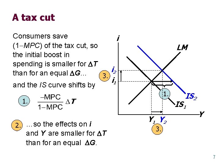
A tax cut Consumers save i (1 MPC) of the tax cut, so the initial boost in spending is smaller for T i 2 than for an equal G… 3. i 1 and the IS curve shifts by LM 1. 2. …so the effects on i and Y are smaller for T than for an equal G. IS 2 IS 1 Y 2 Y 3. 7

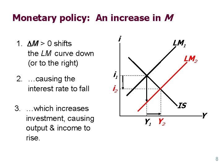
Monetary policy: An increase in M i 1. M > 0 shifts the LM curve down (or to the right) 2. …causing the interest rate to fall 3. …which increases investment, causing output & income to rise. LM 1 LM 2 i 1 i 2 IS Y 1 Y 2 Y 8

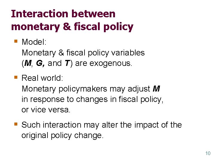
Interaction between monetary & fiscal policy § Model: Monetary & fiscal policy variables (M, G, and T ) are exogenous. § Real world: Monetary policymakers may adjust M in response to changes in fiscal policy, or vice versa. § Such interaction may alter the impact of the original policy change. 10

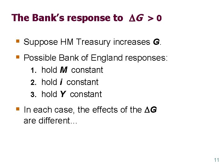
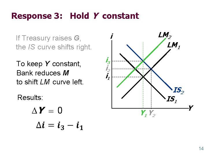
The Bank’s response to G > 0 § Suppose HM Treasury increases G. § Possible Bank of England responses: 1. hold M constant 2. hold i constant 3. hold Y constant § In each case, the effects of the G are different… 11

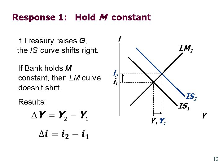
Response 1: Hold M constant If Treasury raises G, the IS curve shifts right. If Bank holds M constant, then LM curve doesn’t shift. i LM 1 i 2 i 1 IS 2 IS 1 Results: Y 1 Y 2 Y 12

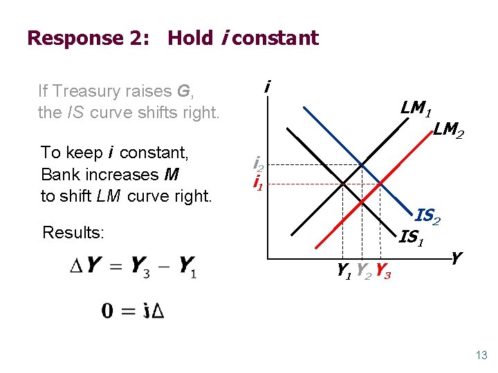
Response 2: Hold i constant If Treasury raises G, the IS curve shifts right. To keep i constant, Bank increases M to shift LM curve right. i LM 1 LM 2 i 1 IS 2 IS 1 Results: Y 1 Y 2 Y 3 Y 13

Response 3: Hold Y constant If Treasury raises G, the IS curve shifts right. To keep Y constant, Bank reduces M to shift LM curve left. LM 2 LM 1 i i 3 i 2 i 1 IS 2 IS 1 Results: Y 1 Y 2 Y 14

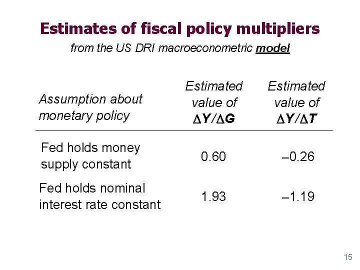
Estimates of fiscal policy multipliers from the US DRI macroeconometric model Assumption about monetary policy Estimated value of Y / G Estimated value of Y / T Fed holds money supply constant 0. 60 0. 26 Fed holds nominal interest rate constant 1. 93 1. 19 15

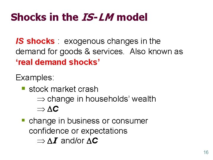
Shocks in the IS -LM model IS shocks : exogenous changes in the demand for goods & services. Also known as ‘real demand shocks’ Examples: § stock market crash change in households’ wealth C § change in business or consumer confidence or expectations I and/or C 16

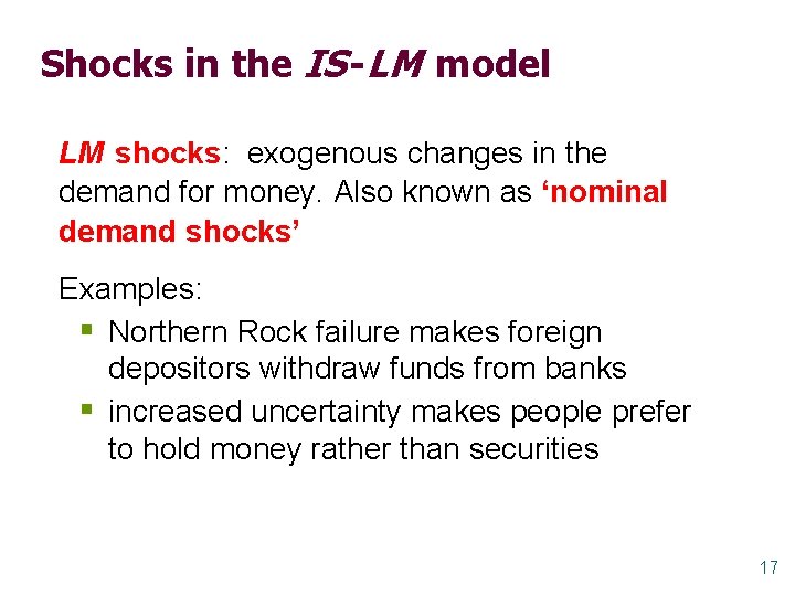
Shocks in the IS -LM model LM shocks: exogenous changes in the demand for money. Also known as ‘nominal demand shocks’ Examples: § Northern Rock failure makes foreign depositors withdraw funds from banks § increased uncertainty makes people prefer to hold money rather than securities 17

Inflation Report August 2013 18

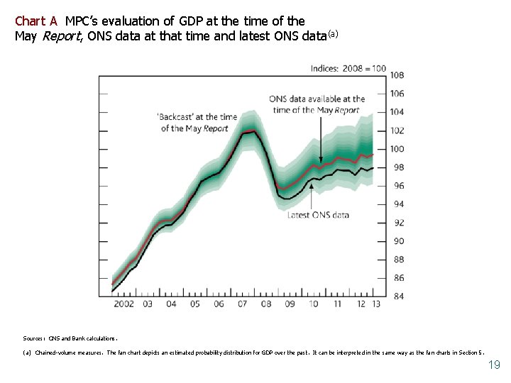
Chart A MPC’s evaluation of GDP at the time of the May Report, ONS data at that time and latest ONS data(a) Sources: ONS and Bank calculations. (a) Chained-volume measures. The fan chart depicts an estimated probability distribution for GDP over the past. It can be interpreted in the same way as the fan charts in Section 5. 19

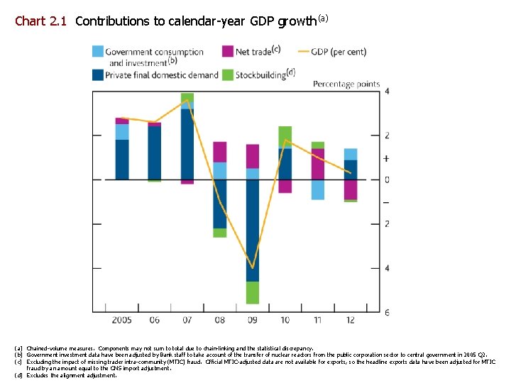
Chart 2. 1 Contributions to calendar-year GDP growth(a) Chained-volume measures. Components may not sum to total due to chain-linking and the statistical discrepancy. (b) Government investment data have been adjusted by Bank staff to take account of the transfer of nuclear reactors from the public corporation sector to central government in 2005 Q 2. (c) Excluding the impact of missing trader intra-community (MTIC) fraud. Official MTIC-adjusted data are not available for exports, so the headline exports data have been adjusted for MTIC fraud by an amount equal to the ONS import adjustment. (d) Excludes the alignment adjustment. 20

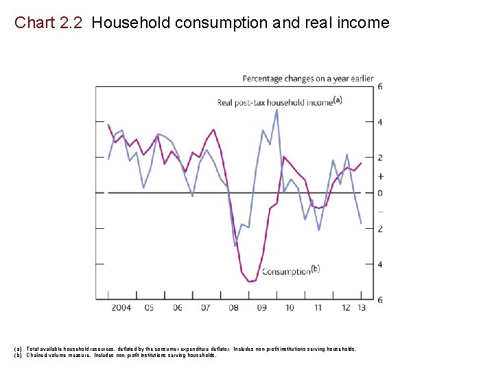
Chart 2. 2 Household consumption and real income (a) Total available household resources, deflated by the consumer expenditure deflator. Includes non-profit institutions serving households. (b) Chained-volume measure. Includes non-profit institutions serving households.

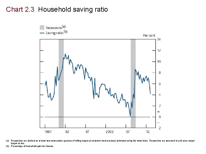
Chart 2. 3 Household saving ratio (a) Recessions are defined as at least two consecutive quarters of falling output (at constant market prices) estimated using the latest data. Recessions are assumed to end once output began to rise. (b) Percentage of household post-tax income.

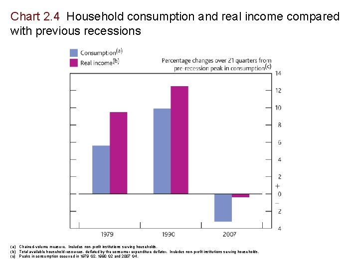
Chart 2. 4 Household consumption and real income compared with previous recessions (a) Chained-volume measure. Includes non-profit institutions serving households. (b) Total available household resources, deflated by the consumer expenditure deflator. Includes non-profit institutions serving households. (c) Peaks in consumption occurred in 1979 Q 2, 1990 Q 2 and 2007 Q 4.

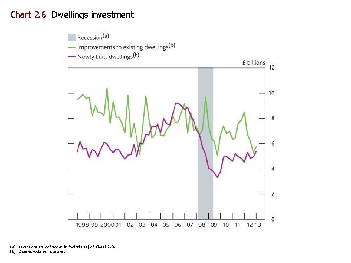
Chart 2. 6 Dwellings investment (a) Recessions are defined as in footnote (a) of Chart 2. 3. (b) Chained-volume measures.

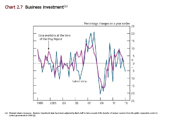
Chart 2. 7 Business investment(a) Chained-volume measures. Business investment data have been adjusted by Bank staff to take account of the transfer of nuclear reactors from the public corporation sector to central government in 2005 Q 2.

Chart 2. 1 Contributions to calendar-year GDP growth(a) Chained-volume measures. Components may not sum to total due to chain-linking and the statistical discrepancy. (b) Government investment data have been adjusted by Bank staff to take account of the transfer of nuclear reactors from the public corporation sector to central government in 2005 Q 2. (c) Excluding the impact of missing trader intra-community (MTIC) fraud. Official MTIC-adjusted data are not available for exports, so the headline exports data have been adjusted for MTIC fraud by an amount equal to the ONS import adjustment. (d) Excludes the alignment adjustment.

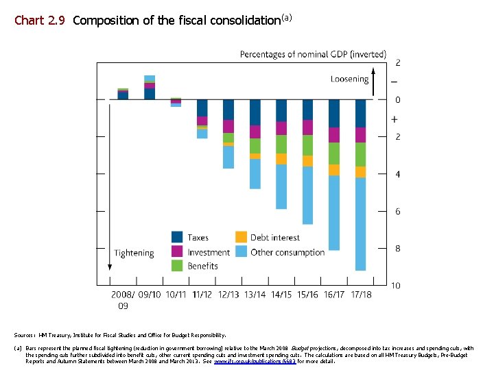
Chart 2. 9 Composition of the fiscal consolidation(a) Sources: HM Treasury, Institute for Fiscal Studies and Office for Budget Responsibility. (a) Bars represent the planned fiscal tightening (reduction in government borrowing) relative to the March 2008 Budget projections, decomposed into tax increases and spending cuts, with the spending cuts further subdivided into benefit cuts, other current spending cuts and investment spending cuts. The calculations are based on all HM Treasury Budgets, Pre-Budget Reports and Autumn Statements between March 2008 and March 2013. See www. ifs. org. uk/publications/6683 for more detail.

29

30

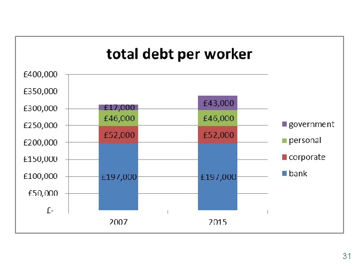
31

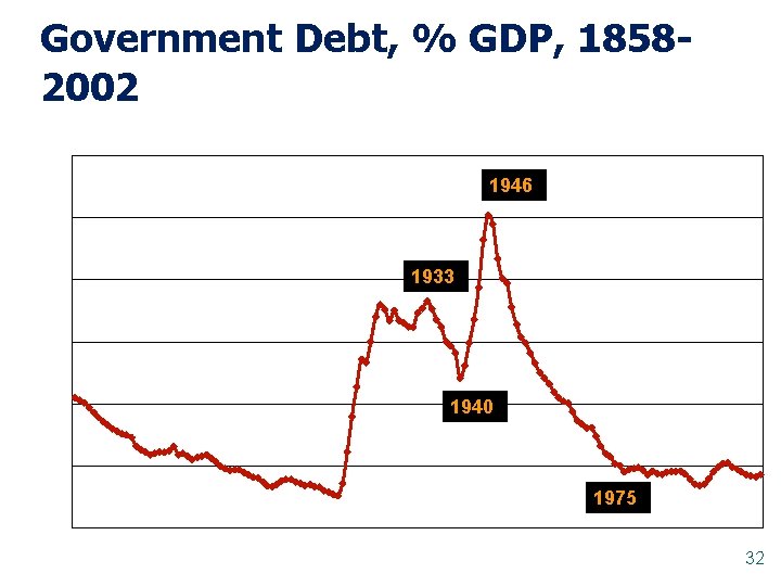
Government Debt, % GDP, 18582002 1946 1933 1940 1975 32

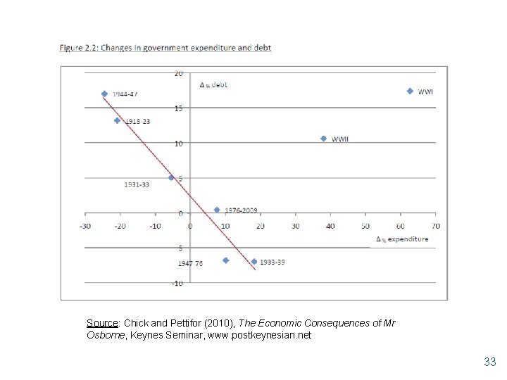
Source: Chick and Pettifor (2010), The Economic Consequences of Mr Osborne, Keynes Seminar, www. postkeynesian. net 33

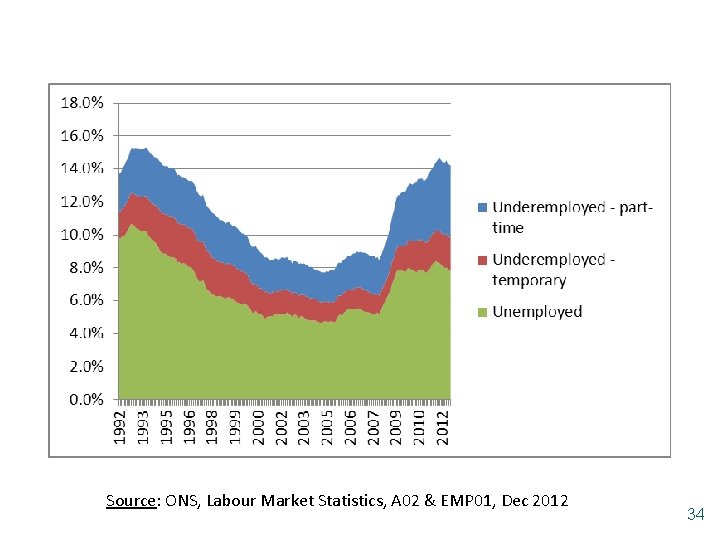
Source: ONS, Labour Market Statistics, A 02 & EMP 01, Dec 2012 34

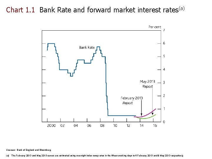
Chart 1. 1 Bank Rate and forward market interest rates(a) Sources: Bank of England Bloomberg. (a) The February 2013 and May 2013 curves are estimated using overnight index swap rates in the fifteen working days to 6 February 2013 and 8 May 2013 respectively.

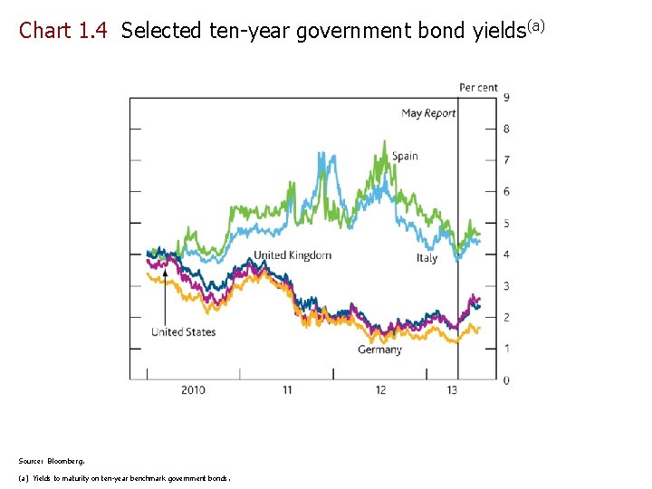
Chart 1. 4 Selected ten-year government bond yields(a) Source: Bloomberg. (a) Yields to maturity on ten-year benchmark government bonds.

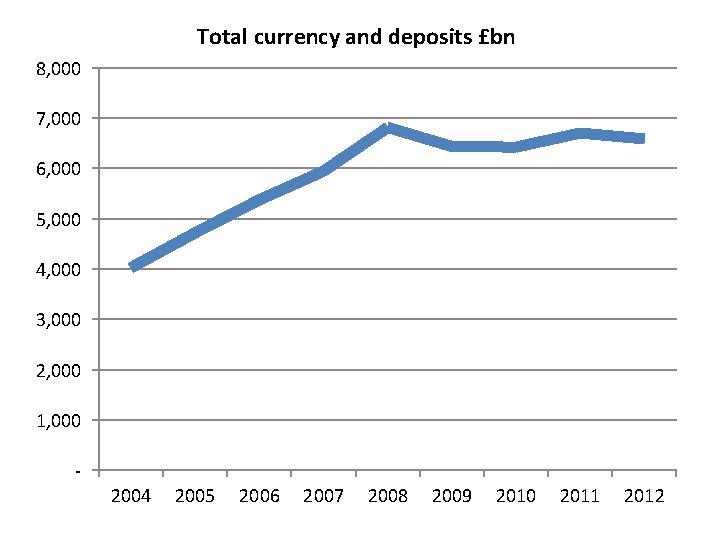
Total currency and deposits £bn 8, 000 7, 000 6, 000 5, 000 4, 000 3, 000 2, 000 1, 000 2004 2005 2006 2007 2008 2009 2010 2011 2012

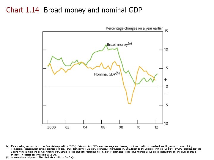
Chart 1. 14 Broad money and nominal GDP (a) M 4 excluding intermediate other financial corporations (OFCs). Intermediate OFCs are: mortgage and housing credit corporations; non-bank credit grantors; bank holding companies; securitisation special purpose vehicles; and other activities auxiliary to financial intermediation. In addition to the deposits of these five types of OFCs, sterling deposits arising from transactions between banks or building societies and ‘other financial intermediaries’ belonging to the same financial group are excluded from this measure of broad money. The latest observation is 2012 Q 2. (b) At current market prices. The latest observation is 2012 Q 1.

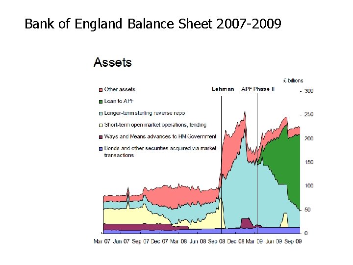
Bank of England Balance Sheet 2007 -2009

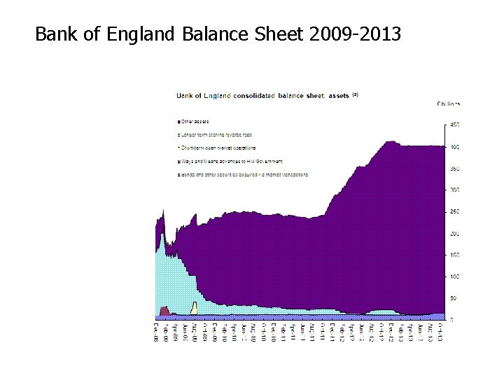
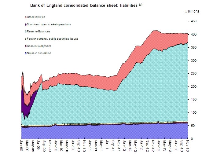
Bank of England Balance Sheet 2009 -2013

Chart 1. 4 Selected ten-year government bond yields(a) Source: Bloomberg. (a) Yields to maturity on ten-year benchmark government bonds.

Other interesting resources • Institute for Fiscal Studies – Excellent analysis and interpretation • Office for Budget Responsibility – Mainly focussed on fiscal position but produces the economic forecasts on which the Budget is based • HM Treasury Budget Website • National Statistics

Summary 1. IS-LM shows how fiscal and monetary policy interact, with the possibility of ‘crowding out’ 2. The monetary policy response to 2008 has been to floor it, including using QE to stop the money supply shrinking and keep long bond rates low. No chance of crowding out. slide 44

Summary 3. However, UK discretionary fiscal policy switched from mildly supportive to contractionary in 2010. 4. Output has stagnated until recently, still several percentage points below 2008. slide 45

Next time Extending the aggregate demand model to take account of foreign trade and the exchange rate slide 46