Diploma Macro Paper 2 Monetary Macroeconomics Lecture 2

Diploma Macro Paper 2 Monetary Macroeconomics Lecture 2 Aggregate demand: Consumption and the Keynesian Cross Mark Hayes slide 1

Outline § Introduction § Map of the AD-AS model slide 2

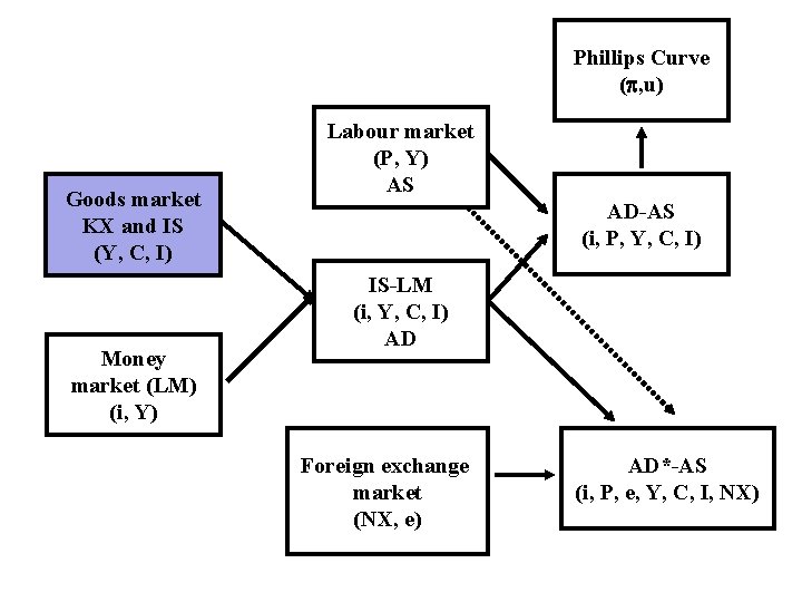
Phillips Curve ( , u) Goods market KX and IS (Y, C, I) Money market (LM) (i, Y) Labour market (P, Y) AS AD-AS (i, P, Y, C, I) IS-LM (i, Y, C, I) AD Foreign exchange market (NX, e) AD*-AS (i, P, e, Y, C, I, NX)

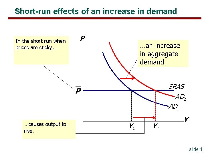
Short-run effects of an increase in demand In the short run when prices are sticky, … P …an increase in aggregate demand… SRAS AD 2 AD 1 …causes output to rise. Y 1 Y 2 Y slide 4

Outline § Introduction § Map of the AD-AS model § This lecture, we begin explaining the AD curve § Step 1: Equilibrium with variable income and consumption - the Keynesian Cross § Various Multipliers slide 5

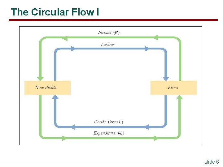
The Circular Flow I slide 6

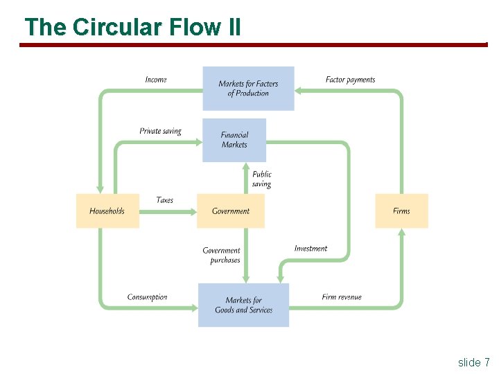
The Circular Flow II slide 7

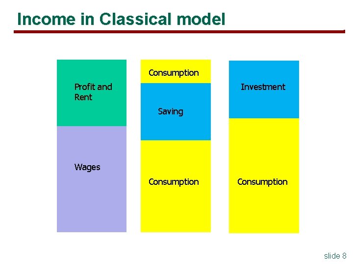
Income in Classical model Consumption Profit and Rent Investment Saving Wages Consumption slide 8

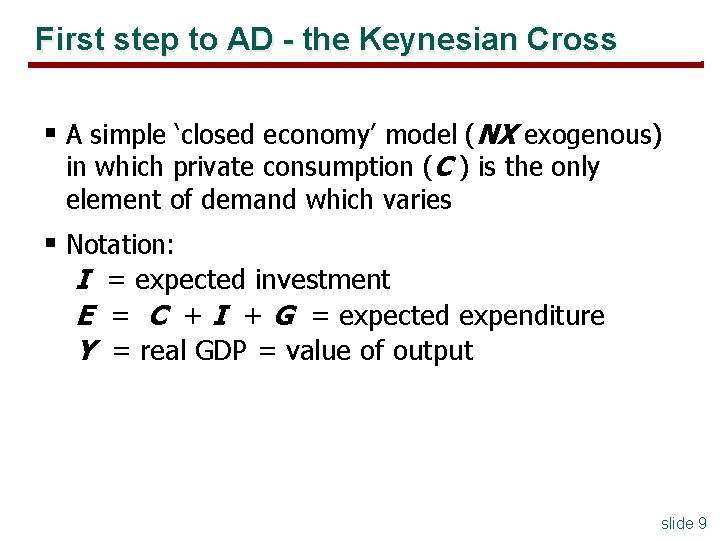
First step to AD - the Keynesian Cross § A simple ‘closed economy’ model (NX exogenous) in which private consumption (C ) is the only element of demand which varies § Notation: I = expected investment E = C + I + G = expected expenditure Y = real GDP = value of output slide 9

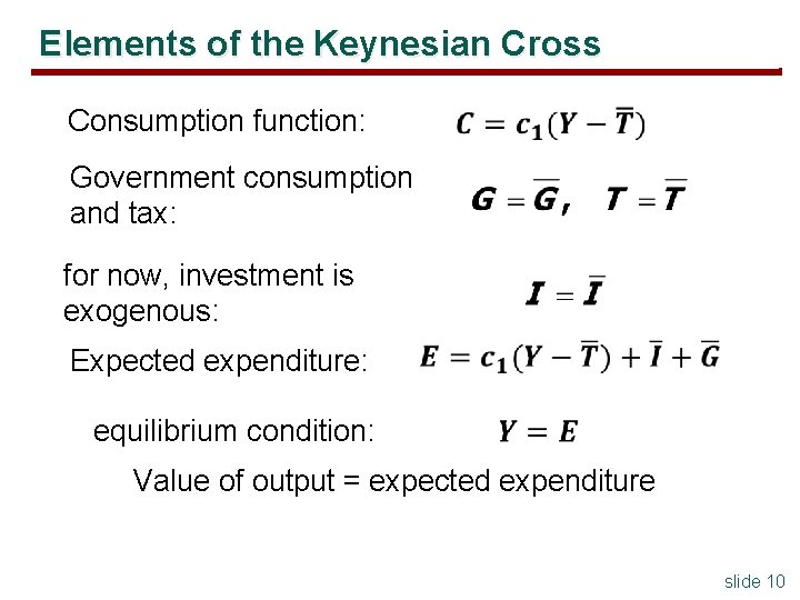
Elements of the Keynesian Cross Consumption function: Government consumption and tax: for now, investment is exogenous: Expected expenditure: equilibrium condition: Value of output = expected expenditure slide 10

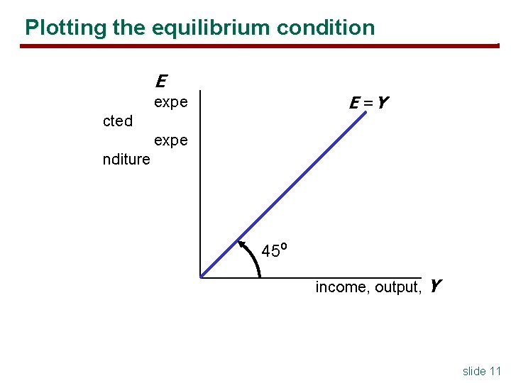
Plotting the equilibrium condition E E =Y expe cted expe nditure 45º income, output, Y slide 11

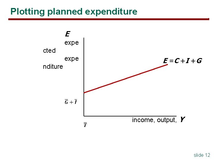
Plotting planned expenditure E expe cted expe nditure E =C +I +G income, output, Y slide 12

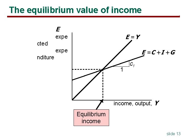
The equilibrium value of income E E =Y expe cted expe E =C +I +G nditure 1 c 1 income, output, Y Equilibrium income slide 13

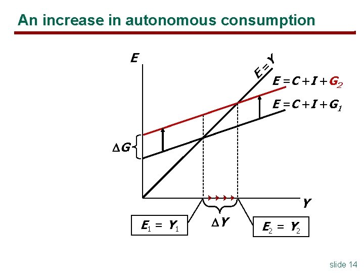
An increase in autonomous consumption = E Y E E =C +I +G 2 E =C +I +G 1 G Y E 1 = Y 1 Y E 2 = Y 2 slide 14

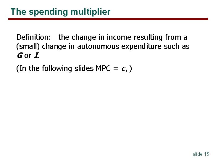
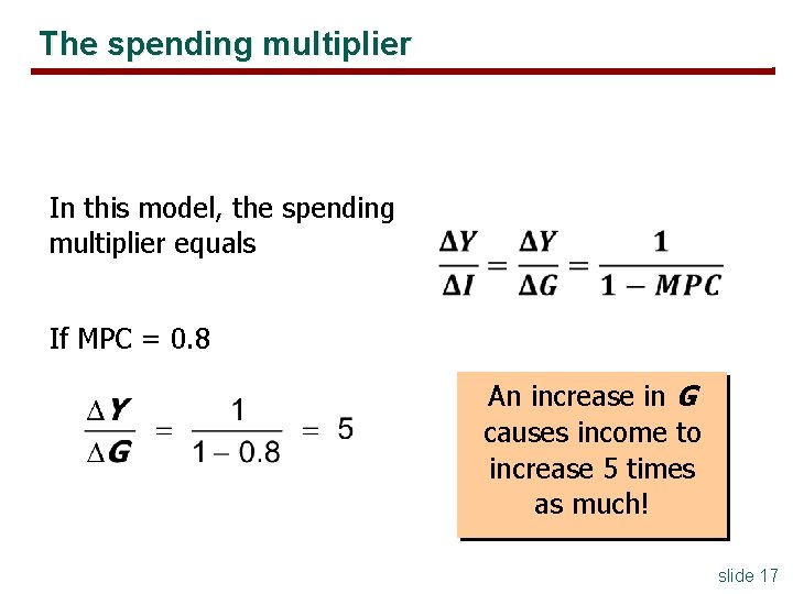
The spending multiplier Definition: the change in income resulting from a (small) change in autonomous expenditure such as G or I. (In the following slides MPC = c 1 ) slide 15

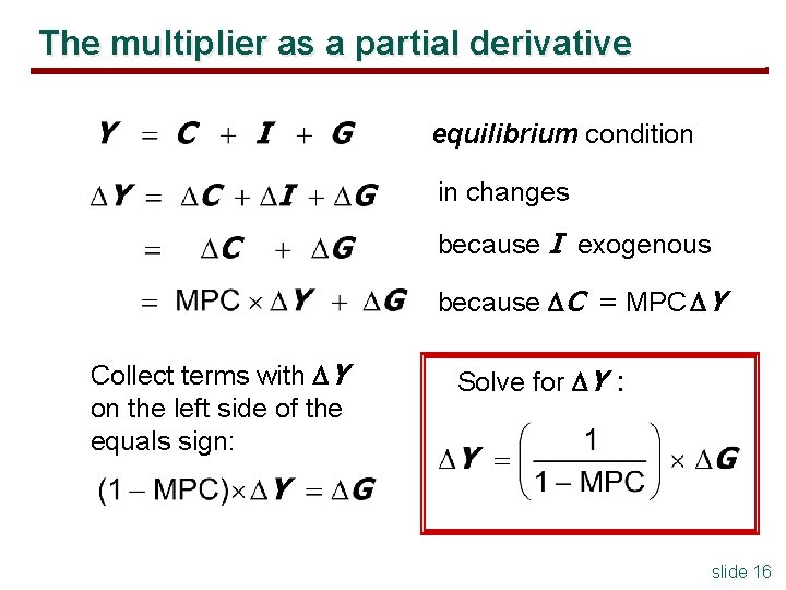
The multiplier as a partial derivative equilibrium condition in changes because I exogenous because C = MPC Y Collect terms with Y on the left side of the equals sign: Solve for Y : slide 16

The spending multiplier In this model, the spending multiplier equals If MPC = 0. 8 An increase in G causes income to increase 5 times as much! slide 17

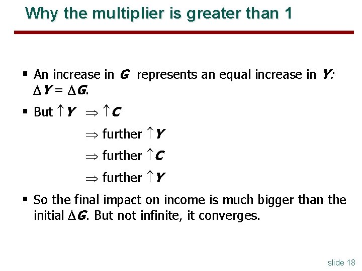
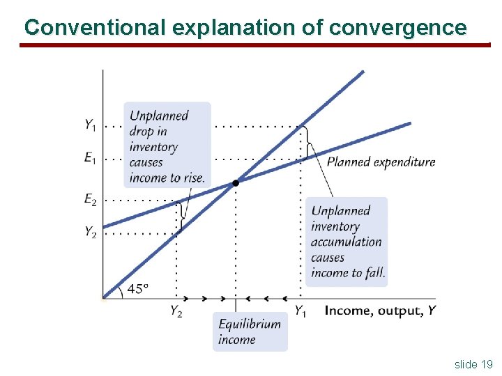
Why the multiplier is greater than 1 § An increase in G represents an equal increase in Y: Y = G. § But Y C further Y further C further Y § So the final impact on income is much bigger than the initial G. But not infinite, it converges. slide 18

Conventional explanation of convergence slide 19

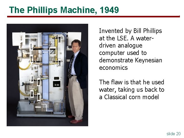
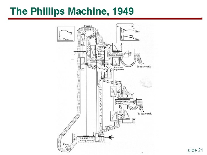
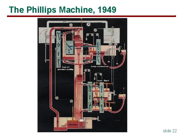
The Phillips Machine, 1949 Invented by Bill Phillips at the LSE. A waterdriven analogue computer used to demonstrate Keynesian economics The flaw is that he used water, taking us back to a Classical corn model slide 20

The Phillips Machine, 1949 slide 21

The Phillips Machine, 1949 slide 22

The Phillips Machine, 1949 www. sms. cam. ac. uk/media/1094078 slide 23

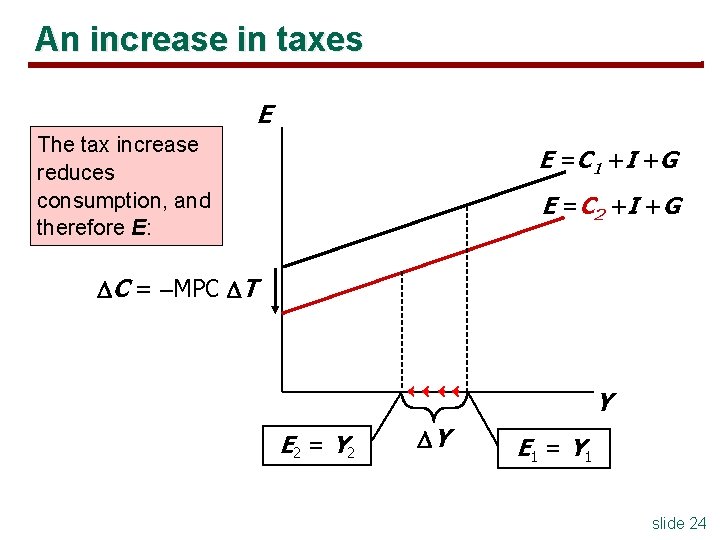
An increase in taxes E The tax increase reduces consumption, and therefore E: E =C 1 +I +G E =C 2 +I +G C = MPC T Y E 2 = Y 2 Y E 1 = Y 1 slide 24

The tax multiplier Definition: the change in income resulting from a (small) change in T slide 25

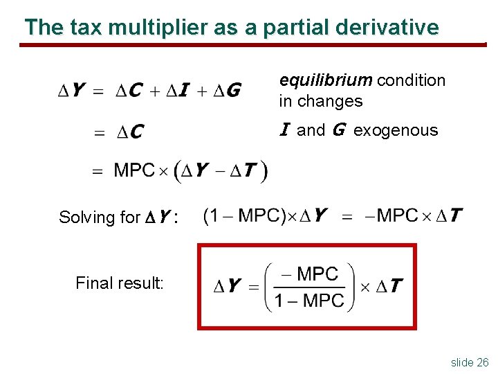
The tax multiplier as a partial derivative equilibrium condition in changes I and G exogenous Solving for Y : Final result: slide 26

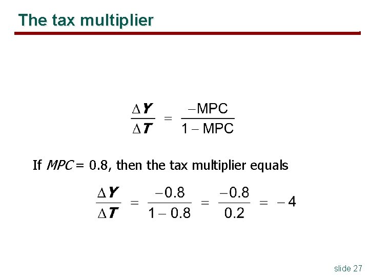
The tax multiplier If MPC = 0. 8, then the tax multiplier equals slide 27

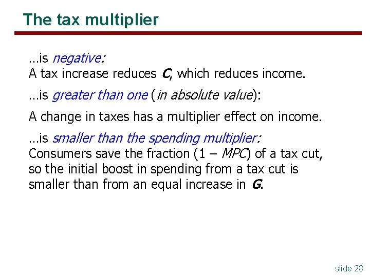
The tax multiplier …is negative: A tax increase reduces C, which reduces income. …is greater than one (in absolute value): A change in taxes has a multiplier effect on income. …is smaller than the spending multiplier: Consumers save the fraction (1 – MPC) of a tax cut, so the initial boost in spending from a tax cut is smaller than from an equal increase in G. slide 28

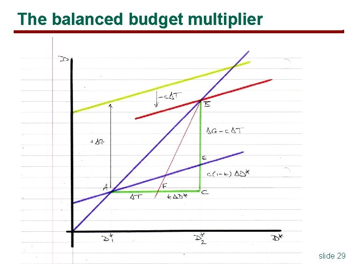
The balanced budget multiplier slide 29

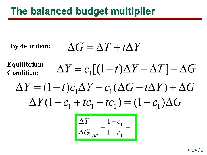
The balanced budget multiplier By definition: Equilibrium Condition: slide 30

Summary § Keynesian cross: equilibrium income determined with income and consumption variable § Shows how the direction of causation between saving and investment is reversed from the Classical model § The multiplier as comparative statics – Spending, tax and balanced budget multipliers – Comparing two equilibrium positions does not explain the dynamic process linking them slide 31

Next time § Step 2 of building the AD curve § Finding equilibrium when income, consumption and investment can all move § the IS-LM model slide 32