Data Science on Medical Data Carlos Ordonez Department

Data Science on Medical Data Carlos Ordonez Department of Computer Science University of Houston, USA

Outline • Motivation Medical data – Exploratory analysis and modeling • Data mining: – Constrained Association Rules – Cube Exploration and Analysis • Machine learning: – Unsupervised: PCA, KM – Supervised: LR, SSVS, NB, Deep neural nets 2/45

Challenges with medical data • Goal: discovering medically significant knowledge, avoid artifacts of combinatorial search • Size: small • Variety of attributes, numeric, categorical, image, text • Medical application: heart disease and cancer 3/45

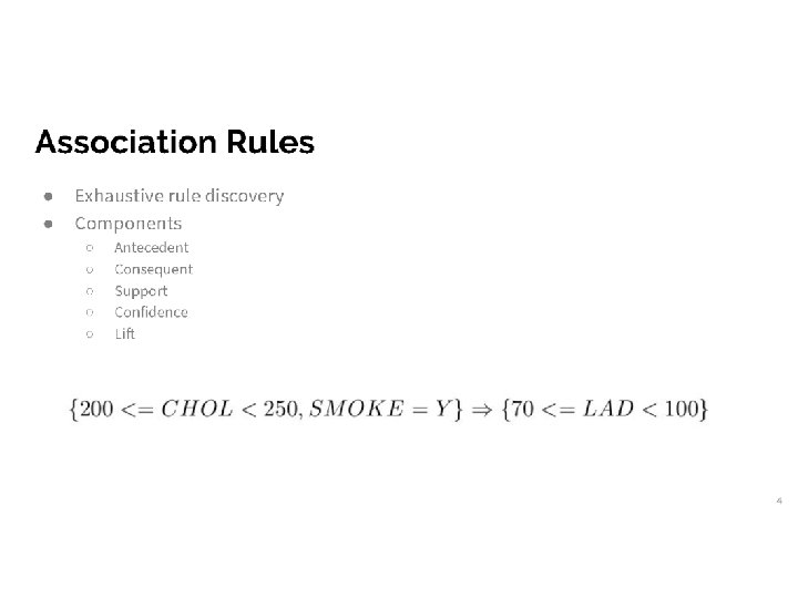
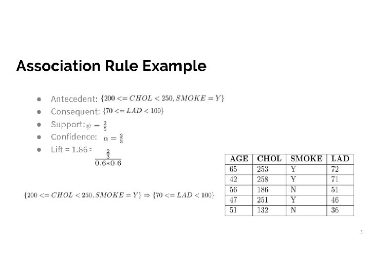
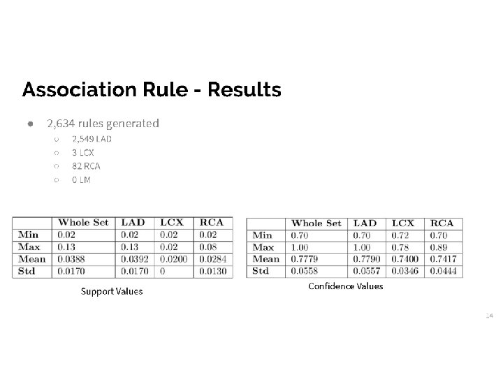
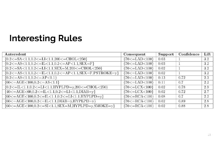
Data mining Constrained Association Rules • Association rules – technique for identifying patterns in datasets using confidence • Looks for relationships between the variables • Detects groups of items that frequently occur together in a given dataset • Rules are in the format X => Y • The set of items X are often found in conjunction with the set of items Y 4/45

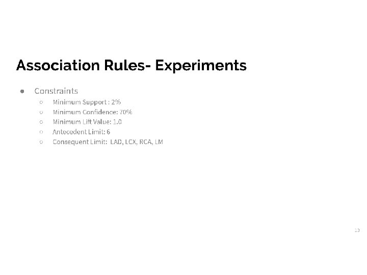
The Constraints • Group Constraint • Determines which variables can occur together in the final rules • Item Constraint • Determines which variables will be used in the study • Allows the user to ignore some variables • Antecedent / Consequent Constraint • Determines the side of the rule that a variable can appear on 5/45

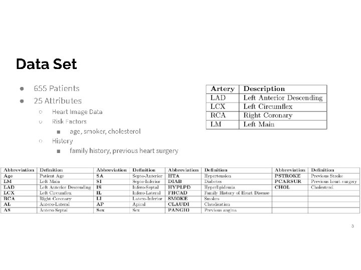
Heart disease data set (artery stenosis) • • Input dataset: p=25, n=655 Three types of Attributes: – P: perfusion measurements – R: risk factor – D: heart disease measurements 6/45

Impact of constraints • . 7/45

No heart disease 8/45

Yes heart disease 9/45

Rule set covers • These figures show some selected cover rules, predicting absence or existence of disease. 10/45

Data mining Cube Exploration • Definition: – Input table F with n records – Cube dimension: D={D 1, D 2, …Dd} – Measure dimension: A={A 1, A 2, …Ae} – In OLAP processing, the basic idea is to compute aggregations on measure Ai by subsets of dimensions G, G D. 11/45

OLAP Exploration and Analysis • Example: – Cube with three dimensions (D 1, D 2, D 3) – Each face represents a subcube on two dimensions – Each cell represent subcube on one dimension 12/45

Cube Statistical Tests • Statistical tests on pairs of OLAP sub cubes to analyze their relationship • Show that a pair of sub cubes are significantly different from each other with a stats basis 13/45

Cube Statistical Tests • The null hypothesis H 0 states 1= 2 and the goal is to find groups where H 0 can be rejected with high confidence 1 -p. • The so called alternative hypothesis H 1 states 1 2. • We use a two-tailed test which allows finding a significant difference on both tail of the Gaussian distribution in order to compare means in any order ( 1 2 or 2 1). • The test relied on the following equation to compute a random variable z. 14/45

Transforming heart data set into cube • • • n = 655 d = 21 e = 4 Includes patient information, habits, and perfusion measurements as dimensions Measures are the stenosis, or amount of narrowing, of the four main arteries of the human heart 15/45

Experiment Evaluation • Heart data set: Group pairs with significant measure differences at p=0. 01 16/45

Experiment Evaluation • Summary of medical result at p=0. 01 • The most important discriminating attributes are OLDYN, SEX and SMOKE. 17/45

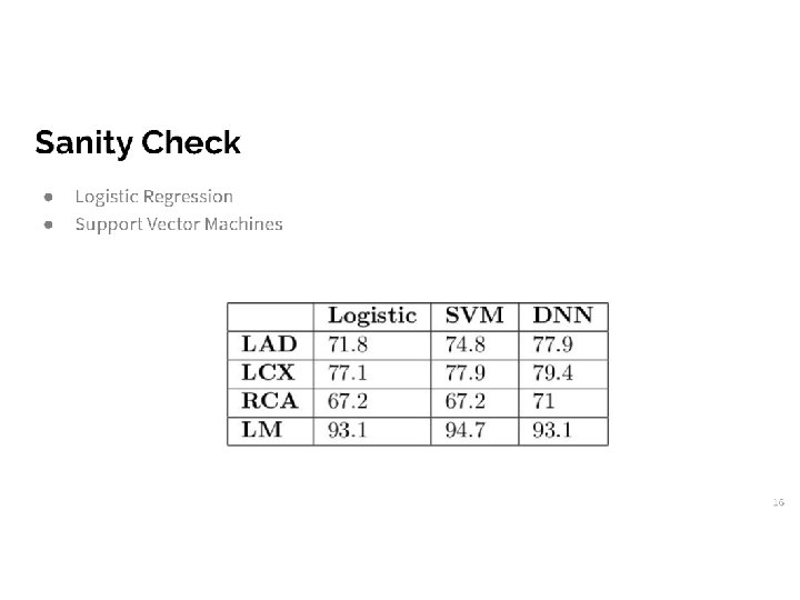
Machine Learning • Unsupervised – PCA – KM • Supervised – Regression: Linear and Logistic – Naïve Bayes (std, class decomposition) – Deep neural nets 18/45

PCA: Principal Component Analysis • Dimensionality reduction technique for highdimensional data (e. g. microarray data). • Exploratory data analysis, by finding hidden relationships between attributes. Assumptions: – Linearity of the data. – Statistical importance of mean and covariance. – Large variances have important dynamics. 19/45

Principal Component Analysis • Rotation of the input space to eliminate redundancy. • Most variance is preserved. • Minimal correlation between attributes. • UTX is a new rotated space. • Select the kth most representative components of U. (k<d) • Solving PCA is equivalent to solve SVD, defined by the eigen-problem: U: left eigenvectors E: the eigenvalues V: the right eigenvectors X=UEVT XXT=UE 2 UT 20/45

PCA: cancer data U 1 age U 2 0. 393 0. 223 gender -0. 293 0. 454 on_thyroxine -0. 161 U 3 U 4 -0. 413 query_thyroxine 0. 229 -0. 100 -0. 397 on_antithyroid_med 0. 107 0. 221 -0. 175 sick 0. 171 pregnant surgery I 131_treatment query_hypothyroid 0. 019 -0. 108 0. 608 0. 195 -0. 226 0. 327 U 7 0. 447 U 8 -0. 405 -0. 100 0. 162 0. 446 0. 184 -0. 204 0. 131 -0. 188 0. 246 0. 138 U 6 -0. 259 0. 232 U 5 0. 208 -0. 846 -0. 194 -0. 276 -0. 214 0. 107 0. 329 0. 360 -0. 059 -0. 157 0. 136 0. 294 -0. 573 -0. 129 0. 189 -0. 251 query_hyperthyroid -0. 223 0. 107 lithium -0. 134 0. 159 0. 421 0. 217 0. 247 0. 319 0. 216 goitre -0. 100 -0. 174 0. 166 -0. 430 0. 236 0. 278 -0. 178 21/45

PCA Example U 1 U 2 U 3 U 4 U 5 U 6 U 7 U 8 age 0. 102 chol 0. 131 0. 175 0. 198 0. 156 claudi 0. 173 0. 252 0. 220 0. 261 0. 305 0. 353 0. 144 -0. 420 0. 266 -0. 193 diab fhcad -0. 273 -0. 408 gender -0. 409 0. 347 -0. 106 0. 379 hta -0. 128 -0. 122 0. 138 0. 109 hyplpd 0. 217 pangio -0. 103 0. 183 0. 195 -0. 204 0. 224 -0. 111 -0. 347 -0. 318 pcarsur 0. 286 pstroke 0. 449 0. 138 -0. 157 smoke 0. 159 -0. 323 0. 417 lad 0. 371 0. 504 lcx 0. 572 -0. 135 -0. 103 -0. 448 -0. 239 -0. 152 0. 105 0. 275 0. 194 0. 217 0. 326 0. 108 0. 393 -0. 105 -0. 110 -0. 154 -0. 311 -0. 415 -0. 117 -0. 217 0. 263 0. 370 0. 152 0. 123 -0. 464 0. 342 -0. 170 -0. 160 -0. 516 0. 448 0. 422 0. 160 0. 205 22/45

Cluster Means and Weights • Means are assigned around the global mean based on Gaussian initialization. • Table below shows means of clusters having 9 dimensions (d). • The weight of a cluster is given by 1. 0/k, where k is the number of clusters. Class Means Weight AGE SEX DIAB HYPLPD FHCAD SMOKE CHOL LA AP 0 60 0. 721 0. 209 0. 116 0. 698 185 -0. 178 -0. 331 0. 0754 0 76. 5 0. 632 0. 08 0. 488 0. 056 0. 488 223 -0. 225 -0. 37 0. 219 0 42. 2 0. 754 0. 029 0. 667 0. 261 0. 58 224 -0. 505 -0. 715 0. 121 0 65. 1 0. 753 0. 193 0. 602 0. 0904 0. 566 223 -0. 22 -0. 375 0. 291 0 56. 5 0. 652 0. 261 0. 217 0. 261 0. 565 139 -0. 379 -0. 527 0. 0404 0 54. 2 0. 729 0. 132 0. 583 0. 104 0. 66 223 -0. 26 -0. 519 0. 253 1 51. 9 0. 533 0. 2 0. 933 0. 267 0. 733 269 0. 0233 -0. 577 0. 176 23/45

Prediction of Accuracy Varying k (Same Clusters k per Class) Dimensions = 21 (Perfusion Measurements + Risk factors) Accuracy for LAD Accuracy for RCA k=2 65. 8% 66. 5% k=4 67. 90% 68. 82% k=6 69. 89% 70. 42% k=8 75. 11% 72. 67% k = 10 68. 35% 70. 23% 24/45

Prediction of Accuracy Varying k (Same Clusters k per Class) Dimensions=9 (Perfusion Measurements) Accuracy for LAD Accuracy for RCA k=2 73. 13% 67. 63% k=4 73. 37% 67. 90% k=6 74. 80% 69. 80% k=8 77. 07% 72. 06% k = 10 72. 34% 68. 93% 25/45

Machine learning: Linear Regression • There are two main applications for linear regression: Prediction or forecasting of the output or variable of interest Y • Fit a model from the observed Y and the input variables X. • For values of X given without its accompanying value of Y, the model can be used to make a prediction of the output of interest Y. • Given an input data X={x 1, x 2, …, xn}, with d dimensions Xa, and the response or variable of interest Y. • Linear regression finds a set of coefficients β to model: Y = β 0+β 1 X 1+…+βd. Xd+ɛ. 26/45

Bayesian Variable Selection in Linear Regression with SSVS • Bayesian variable selection Quantify the strength of the relationship between Y and a number of explanatory variables Xa. • Assess which Xa may have no relevant relationship with Y. • Identify which subsets of the Xa contain redundant information about Y. • The goal is to find the subset of explanatory variables Xγ which best predicts the output Y, with the regression model Y = βγ Xγ+ɛ. • We use Gibbs sampling, which is an MCMC algorithm, to estimate the probability distribution π(γ|Y, X) of a model to fit the output variable Y. • Other techniques, like stepwise variable selection, perform a partial search to find the model that better explains the output variable. • Stochastic Search Variable Selection finds best “likely” subset of variables based on posterior probabilities. 27/45

Bayesian var. selection in linear regression: heart Variables Gamma Parameters age 1 Variables: 21 chol 2 n = 655 claudi 3 Y: rca Y: lad diab 4 c = 100 fhcad 5 it = 10000 gender 6 burn =1000 hta 7 hyplpd 8 Gamma pangio 9 0, 1, 3, 8, 12, 13, 16, 19 0. 012333 0. 826227 0, 1, 14, 18 0. 061556 0. 768594 pcarsur 10 0, 1, 3, 8, 12, 13 0. 011778 0. 838421 0, 1, 13, 14, 18 0. 028556 pstroke 11 0, 1, 3, 6, 8, 12, 13 0. 011556 0. 832125 0, 1, 8, 14, 18 0. 022889 0. 765396 smoke 12 0, 1, 3, 6, 8, 12, 13, 17 0. 010333 0. 826885 0, 1, 9, 14, 18 0. 014444 0. 766478 il 13 0, 1, 6, 14, 18 0. 013222 0. 766782 ap 14 0, 1, 3, 14, 18 0. 011667 0. 767118 al 15 0, 1, 14, 16, 18 0. 010111 0. 767645 la 16 0, 1, 14, 17, 18 0. 01 0. 767105 as_ 17 0, 1, 14, 18, 21 0. 008667 0. 768276 sa 18 0, 1, 8, 13, 14, 18 0. 008333 0. 762457 Prob r. Squared 0, 1, 3, 8, 9, 12, 13, 16, 19 0. 008889 0. 821647 0, 1, 3, 6, 8, 9, 12, 13 0. 008 0. 826993 0, 1, 3, 8, 12, 13, 17 0. 007222 0. 833006 0, 1, 3, 6, 8, 13, 17 0. 006889 0. 833852 0, 1, 3, 6, 8, 9, 13 0. 006778 0. 838573 0, 1, 3, 6, 8, 9, 12, 13, 17 0. 006556 0. 821839 Gamma Prob r. Squared 0. 7652 28/45

Bayesian variable selection in LR: cancer Cancer microarray data, where gamma are the gene numbers. Gamma Parameters Probability r. Squared 0, 3, 4, 52, 99, 196, 287, 1833, 1857, 2115, 2563, 2601, 3720, 3924, 4854, 4879 0. 761239 0. 00664 0, 3, 4, 52, 99, 196, 287, 1833, 1857, 2563, 2601, 3924, 4854, 4879 0. 108891 0. 006756 dimensions 0, 3, 4, 52, 99, 196, 287, 1833, 1857, 2115, 2563, 2601, 3924, 4854, 4879 0. 050949 0. 006702 n 0, 3, 4, 52, 99, 196, 287, 1833, 3924, 4854, 4879 0. 041958 0. 006771 0, 3, 4, 52, 99, 196, 287, 1833, 2563, 2601, 3924, 4854, 4879 0. 027972 0. 006758 0, 3, 4, 52, 99, 196, 287, 1833, 4854 0. 002997 0. 006836 0, 3, 4, 52, 99, 196, 287, 1833, 4854, 4879 0. 001998 0. 006776 0, 3, 4, 52, 99, 196, 287, 1833, 2601, 3924, 4854, 4879 0. 001998 0. 006758 0, 3, 4, 99, 196, 287, 1833, 4854 0. 000999 0. 006924 d(γ 0) iterations 1 4918 295 1000 c y 1 Cens 29/45

SSVS in the DBMS • • • Bayesian variable selection is implemented completely inside a DBMS with SQL and UDFs for efficient use of memory and processor resources. Our algorithms and storage layouts for tables in the DBMS have a representative impact on execution performance. Compared to the statistical package R, our implementations scale to large data sets: best available 30/45

Logistic Regression (completeness and relationship to neural nets) Similar to linear regression. The data is fitted to a logistic curve. This technique is used for the prediction of probability of occurrence of an event. P(Y=1|x) = π(x) =1/(1+e-g(x)) , where g(x)= β 0+β 1 X 1+β 2 X 2+…+βd. Xd 31/45

Logistic Regression Name med 655 Intercept Train • n = 491 • d = 15 • y = LAD>=70% Test • n = 164 Coefficient Name -2. 191237293 LI Coefficient -0. 090759713 AGE 0. 035740648 LA -0. 210152957 SEX 0. 40150077 AP 0. 600745945 HTA 0. 279865571 AS_ 0. 264413463 DIAB 0. 060630279 SA 0. 342609744 CHOL 0. 001882748 SI 0. 04750216 SMOKE AL 0. 31437235 IS_ 0. 198138067 IL -0. 159692182 0. 446180853 Accuracy med 655 Global Class-0 Class-1 70 74 67 32/45

Naïve Bayes (NB) • • Naïve Bayes is one of the most popular classifiers Easy to understand. Produces a simple model structure. It is robust and has a solid mathematical background. • Can be computed incrementally. • Classification is achieved in linear time. • However, it has an independence assumption. 33/45

Improving Naive Bayes: Class Decomposition • Why Bayesian: – A Bayesian approach to deal with variable independence assumption based on Class Decomposition Using EM Clustering. – Robust models with good accuracy and low overfit. – Classifier adapted to skewed distributions and overlapping set of data points by building local models based on clusters. – EM Algorithm used to fit the mixtures per class. – Bayesian Classifier is composed of a mixture of k distributions or clusters per class. 34/45

Bayesian Classifier Based on K-Means (BKM) • Motivation – Bayesian Classifiers are accurate and efficient. – A Generalization of the Naïve Bayes algorithm. – Model accuracy can be tuned varying number of clusters, setting class priors and making a probabilitybased decision. – EM is a distance based clustering algorithm. – Two phases involved in building the predictive model • Building the predictive model. • Scoring a new data set based on the computed predictive model. 35/45

Heart disease data set • Medical Dataset is used with 655 rows n with varying number of clusters k. • This Dataset has 25 dimensions d which includes diseases to be predicted, risk factors and perfusion measurements. • Dimensions having null values have been replaced with the mean of that dimension. • Here, we predict accuracy for LAD, RCA (2 diseases). • Accuracy is good for maximum k = 8. 36/45

Classification results: heart data set med 655 • n = 655 • d = 15 • g= 0, 1 • G represents if the patient developed heart disease or not. wbcancer • n = 569 • d = 7 • g= 0, 1 • G represents if the cancer is benign or malignant. • Features describe the characteristics of cell nuclei obtained from image of breast mass. Accuracy % med 655 NB 67 83 53 BKM 62 53 70 wbcancer NB 93 91 95 BKM 93 84 97 Global Class-0 Class-1 37/45

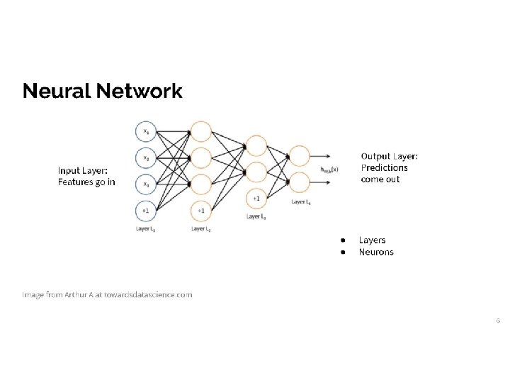
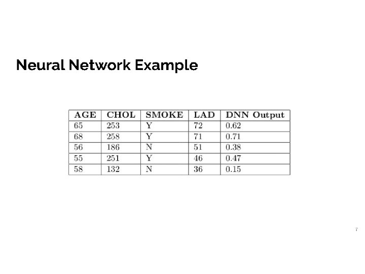
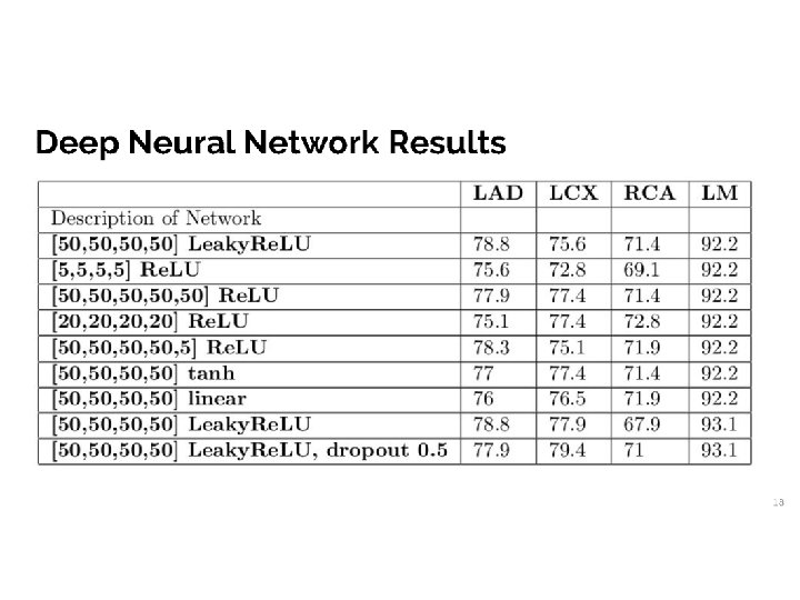
Deep Neural Nets on Medical Data